Image Processing in OpenCV

1 Changing Colorspaces

1.1 目标

• 学习如何将图像从一个颜色空间（color-space）转换到另一个颜色空间，比如，BGR <-> Gray, BGR <-> HSV等。
• 创建一个应用，使之可以提取视频中的有色物体（colored object)
• 学习函数：cv2.cvtColor(), cv2.inRange()等

1.2 改变颜色空间

OpenCV中有超过150种颜色空间转换方法。但这里我们只看两种应用最广泛的，BGR <-> Gray 和 BGR <-> HSV。

注意：
HSV(Hue, Saturation, Value)是根据颜色的直观特性由A. R. Smith在1978年创建的一种颜色空间, 也称六角锥体模型(Hexcone Model)。这个模型中颜色的参数分别是：色调（H），饱和度（S），明度（V）。

对于颜色转换，我们利用函数cv2.cvtColor(input_image, flag)，其中，flag决定转换类型。

BGR -> Gray转换可以用的flag为cv2.COLOR_BGR2GRAY. 相似的，BGR -> HSV，可以用cv2.COLOR_BGR2HSV. 如果想得到其它的flags，可以运行下面的命令：

import cv2

flags = [i for i in dir(cv2) if i.startswith('COLOR_')]
print(flags)

注意：
对于HSV来说，Hue范围是[0, 179]， Saturation范围是[0, 255]，Value范围是[0, 255]。不同的软件用不同的刻度（scales）。所以当你比较它们的OpenCV值，你需要标准化它们的范围。

1.3 对象跟踪（Object Tracking）

现在我们知道如何将图像从BGR转换为HSV，我们可以提取有颜色的对象。相比在RGB颜色空间中，在HSV颜色空间中表示颜色更加简单。在我们的应用中我们将提取一个蓝色对象。下面是方法：

• 提取视频的每一帧
• 从BGR空间转换到HSV空间
• 我们对HSV图像在蓝色范围内设定阈值
• 提取蓝色对象，我们可以在图像上做任何想做的事

下面是推荐的代码：

import cv2
import numpy as np

cap = cv2.VideoCapture(0)

while(1):
    # Take each frame
    _, frame = cap.read()
    
    # Convert BGR to HSV
    hsv = cv2.cvtColor(frame, cv2.COLOR_BGR2HSV)
    
    # define range of blue color in HSV
    lower_blue = np.array([110, 50, 50])
    upper_blue = np.array([130, 255, 255])
    
    # Threshold the HSV image to get only blue colors
    # A binary mask is returned, where white pixels represent pixels that fall into the upper and lower limit range and black pixels do not
    mask = cv2.inRange(hsv, lower_blue, upper_blue)
    
    # Bitwise-AND mask and original image
    # 函数原型：bitwise_and(src1, src2, dst=None, mask=None)
    res = cv2.bitwise_and(frame, frame, mask=mask)
    
    cv2.imshow('frame', frame)
    cv2.imshow('mask', mask)
    cv2.imshow('res', res)
    k = cv2.waitKey(1000) & 0xFF
    if k == 27:
        break
        
cv2.destroyAllWindows()

下面的图像显示了蓝色对象的跟踪：

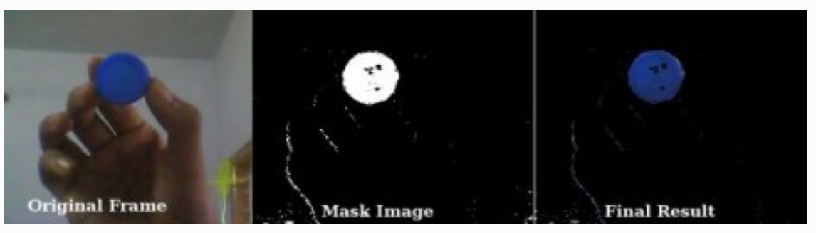
注意：
图像中有一些噪音，我们将在下一章学习如何移除它们。

注意：
这是图像跟踪中最简单的方法。一旦你学习了contours函数，你可以做很多事情，比如，找到这个对象的中心点（centroid）和追踪对象，仅仅通过在摄像头前面移动你的手来画图表，还有许多其它好玩的事情。

1.4 如何找到要跟踪对象的HSV值

这是一个在stackoverflow中可以找到的普遍问题，非常简单，你同样可以用函数cv2.cvtColor()。不用传递图像，而仅仅传递你想要的BGR值。例如，找到绿色的HSV，尝试下面的代码：

import numpy as np
import cv2 

green = np.uint8([[[0, 255, 0]]])
hsv_green = cv2.cvtColor(green, cv2.COLOR_BGR2HSV)
print(hsv_green)

# 输出：[[[ 60 255 255]]]

现在我们取[H-10,100,100]和[H+10,255,255]分别作为下界和上界。除了这个方法，你可以利用如GIMP的图像编辑工具或者线上转换器来找到这些值，但是不要忘记调整HSV范围。

2 Image Thresholding

2.1 目标

• 学习简单的阈值化，自适应阈值化（Adaptive thresholding），Otsu's阈值化等
• 学习函数：cv2.threshold, cv2.adaptiveThreshold等

2.2 简单阈值化

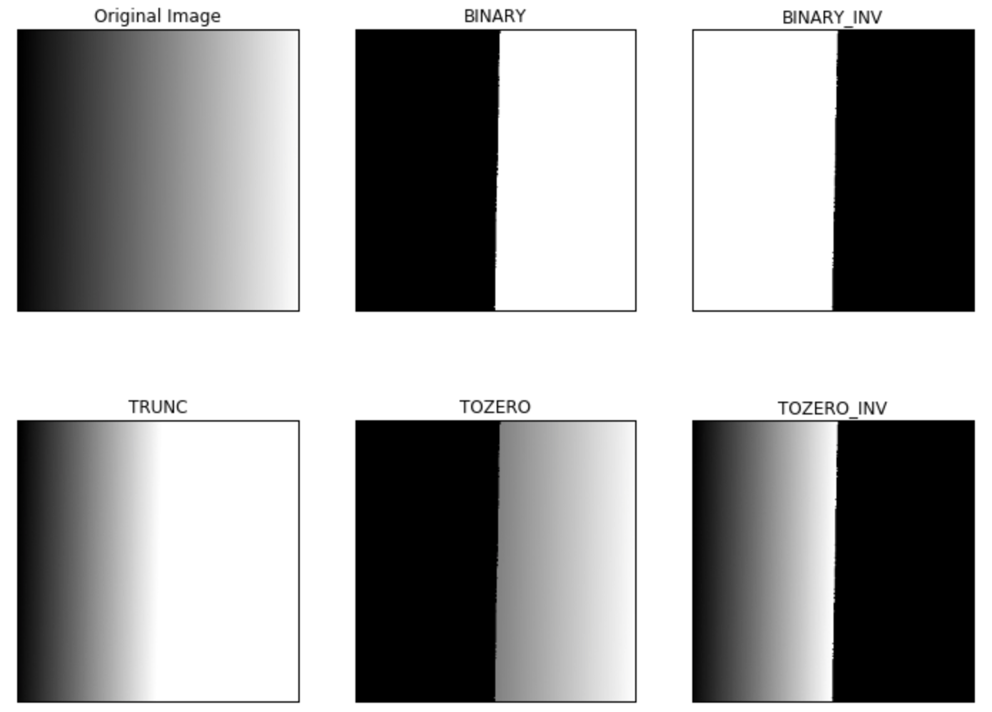
在这里，事情是直截了当的。如果像素值大于阈值，则为其分配一个值（可能是白色），否则为其分配另一个值（可能是黑色）。使用的函数是cv2.threshold。

• 第一个参数是源图像，它应该是灰度图像。
• 第二个参数是用于对像素值进行分类的阈值。
• 第三个参数是maxVal，它表示如果像素值大于（有时小于）阈值则要给定的值。
• 第四个参数是阈值化类型。OpenCV提供不同类型的阈值化，不同的类型是：
  • cv2.THRESH_BINARY
  • cv2.THRESH_BINARY_INV
  • cv2.THRESH_TRUNC
  • cv2.THRESH_TOZERO
  • cv2.THRESH_TOZERO_INV

文件清楚的解释了每种类型意味着什么，可以去查询文件。

输出结果又两个值，第一个是retval，第二个是thresholded image。

import cv2
import numpy as np
from matplotlib import pyplot as plt

img = cv2.imread('gradient.png', 0)
ret, thresh1 = cv2.threshold(img, 127, 255, cv2.THRESH_BINARY)
ret, thresh2 = cv2.threshold(img, 127, 255, cv2.THRESH_BINARY_INV)
ret,thresh3 = cv2.threshold(img,127,255,cv2.THRESH_TRUNC)
ret,thresh4 = cv2.threshold(img,127,255,cv2.THRESH_TOZERO)
ret,thresh5 = cv2.threshold(img,127,255,cv2.THRESH_TOZERO_INV)

titles = ['Original Image', 'BINARY', 'BINARY_INV', 'TRUNC', 'TOZERO', 'TOZERO_INV']
images = [img, thresh1, thresh2, thresh3, thresh4, thresh5]

plt.rcParams['figure.figsize'] = (12, 9)
for i in range(6):
    plt.subplot(2, 3, i+1)
    plt.imshow(images[i], 'gray')
    plt.title(titles[i])
    plt.xticks([])
    plt.yticks([])

plt.show()

2.3 自适应阈值化（Adaptive Thresholding）

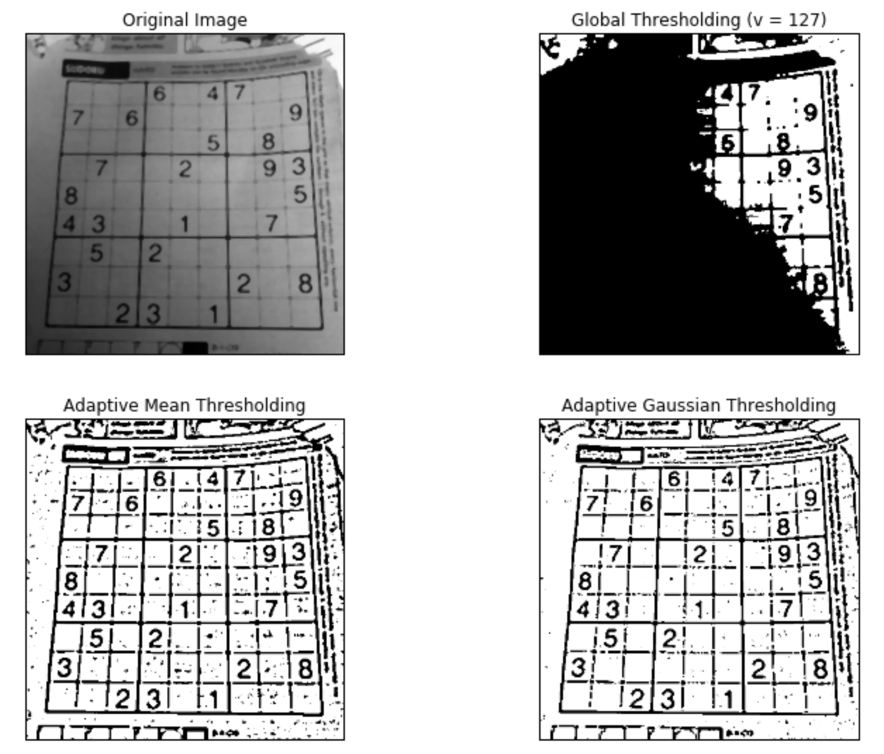
在上一节中，我们使用全局值作为阈值。但是图像在不同区域具有不同照明条件的所有情况下使用全局值可能并不好。在那种情况下，我们进行自适应阈值化处理。在此，算法对图像的小区域计算阈值。因此，我们在同一图像的不同区域获得不同的阈值，它为具有不同照明的图像提供了更好的结果。

它有三个”特殊“的输入参数和一个输出参数。

Adaptive Method - 决定阈值化值如何计算。

• cv2.ADAPTIVE_THRESH_MEAN_C: 阈值是相邻区域的均值
• cv2.ADAPTIVE_THRESH_GAUSSIAN_C: 阈值是邻域值的加权和，其中权重是高斯窗口

Block Size - 决定相邻区域的大小（为正方形邻域）。

C - 它只是从计算的平均值或加权平均值中需要减去的常数。

下面的代码是对于不同照明的图像比较了全局阈值化和自适应阈值化。

import cv2
import numpy as np
from matplotlib import pyplot as plt

img = cv2.imread('dave.jpg', 0)
img = cv2.medianBlur(img, 5)

ret,th1 = cv2.threshold(img, 127, 255, cv2.THRESH_BINARY)
# Block Size = 11, C = 2
th2 = cv2.adaptiveThreshold(img, 255, cv2.ADAPTIVE_THRESH_MEAN_C,
            cv2.THRESH_BINARY, 11, 2)
th3 = cv2.adaptiveThreshold(img, 255, cv2.ADAPTIVE_THRESH_GAUSSIAN_C,
            cv2.THRESH_BINARY, 11, 2)

titles = ['Original Image', 'Global Thresholding (v = 127)',
            'Adaptive Mean Thresholding', 'Adaptive Gaussian Thresholding']
images = [img, th1, th2, th3]

for i in range(4):
    plt.subplot(2, 2, i+1)
    plt.imshow(images[i], 'gray')
    plt.title(titles[i])
    plt.xticks([])
    plt.yticks([])
plt.show()

2.4 Otsu's Binarization（Otsu's二值化）

在上一节中，我告诉你第二个参数是retVal。当我们选择Otsu's二值化时就可以使用了。所以它是什么？

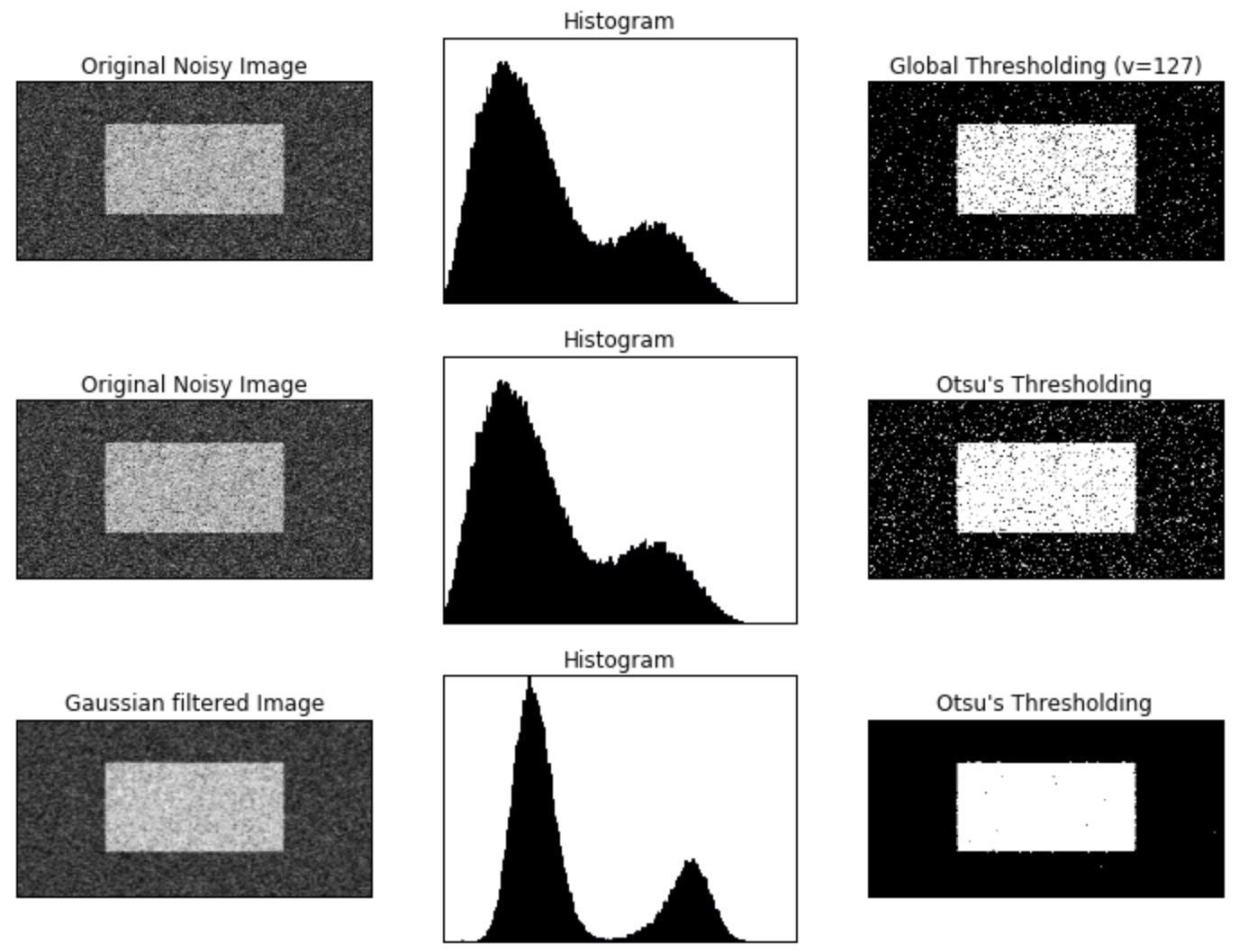
在全局阈值化处理中，我们使用任意值作为阈值，对吗？那么，我们如何知道我们选择的值是好还是不好？答案是，试错法。但考虑双峰图像（bimodal image，简单来说，双峰图像是直方图有两个峰值的图像），我们可以将这些峰值中间的值近似作为阈值，对吧？这就是Otsu二值化的作用。因此，简单来说，它会根据双峰图像的图像直方图自动计算阈值。（对于非双峰图像，二值化不准确。）

为此，我们使用cv2.threshold()函数，但传递了一个额外的flag，cv2.THRESH_OTSU。对于阈值，只需传递零。然后算法找到最优阈值并返回第二个输出retVal。如果未使用Otsu阈值化，则retVal与你使用的阈值相同。

请查看以下示例，输入图像是噪音图像。在第一种情况下，我使用全局阈值127。在第二种情况下，我直接应用了Otsu阈值化。在第三种情况下，我使用5x5高斯核过滤图像以消除噪声，然后应用Otsu阈值化。了解噪声过滤如何改善结果。

import cv2
import numpy as np
from matplotlib import pyplot as plt

img = cv2.imread('noisy2.png',0)

# global thresholding
ret1, th1 = cv2.threshold(img, 127, 255, cv2.THRESH_BINARY)

# Otsu's thresholding
ret2, th2 = cv2.threshold(img, 0, 255, cv2.THRESH_BINARY + cv2.THRESH_OTSU)

# Otsu's thresholding after Gaussian filtering
blur = cv2.GaussianBlur(img, (5, 5), 0)
ret3, th3 = cv2.threshold(blur, 0, 255, cv2.THRESH_BINARY + cv2.THRESH_OTSU)

# plot all the images and their histograms
images = [img, 0, th1,
          img, 0, th2,
          blur, 0, th3]
titles = ['Original Noisy Image','Histogram','Global Thresholding (v=127)',
          'Original Noisy Image','Histogram',"Otsu's Thresholding",
          'Gaussian filtered Image','Histogram',"Otsu's Thresholding"]

for i in range(3):
    plt.subplot(3,3,i*3+1), plt.imshow(images[i*3], 'gray')
    plt.title(titles[i*3]), plt.xticks([]),  plt.yticks([])
    plt.subplot(3,3,i*3+2), plt.hist(images[i*3].ravel(), 256)
    plt.title(titles[i*3+1]), plt.xticks([]), plt.yticks([])
    plt.subplot(3,3,i*3+3), plt.imshow(images[i*3+2], 'gray')
    plt.title(titles[i*3+2]), plt.xticks([]), plt.yticks([])

plt.show()

2.5 Otsu's二值化是如何工作的

本节演示了Otsu二值化的Python实现，以展示它的实际工作原理。

由于我们正在使用双峰图像，因此Otsu的算法试图找到一个阈值（t），它最小化了给出的如下关系的加权类内方差（weighted within-class variance）：

[sigma_omega^2 = q_1(t)sigma_1^2 + q_2(t)sigma_2^2(t) ]

这里

[q_1(t) = sumlimits_{i=1}^{t} P(i)quad & quad q_2(t) = sumlimits_{i=t+1}^{I}P(i) ]

[mu_1(t) = sum_{i=1}^{t} frac{iP(i)}{q_1(t)} quad & quad mu_2(t) = sum_{i=t+1}^{I} frac{iP(i)}{q_2(t)} ]

[sigma_1^2(t) = sum_{i=1}^{t}[i - mu_1(t)]^2 frac{P(i)}{q_1(t)} quad & quad sigma_2^2(t) = sum_{i=t+1}^{I}[i - mu_2(t)]^2 frac{P(i)}{q_2(t)} ]

以上公式在概率上很容易得到解释：

• (t)是我们要找的阈值；
• (P(i))是像素值(i)在所有像素中出现的概率，所以(q_1(t))是像素值(leq t)的概率，(q_2(t))是像素值(geq t+1)的概率；
• (mu_1(t))是像素值(leq t)的均值，(mu_2(t))是像素值(geq t+1)的均值；
• (sigma_1^2(t))是像素值(leq t)的方差，(sigma_1^2(t))是像素值(geq t+1)的方差。

它实际上找到了一个位于两个峰之间的t值，这个t值使两个类的方差都是最小的。它可以简单地在Python中实现，如下所示：

img = cv2.imread('noisy2.png',0)
blur = cv2.GaussianBlur(img,(5,5),0)

# find normalized_histogram, and its cumulative distribution function
hist = cv2.calcHist([blur],[0],None,[256],[0,256])
hist_norm = hist.ravel()/hist.max()
Q = hist_norm.cumsum()

bins = np.arange(256)

fn_min = np.inf
thresh = -1

for i in range(1,256):
    p1,p2 = np.hsplit(hist_norm,[i]) # probabilities
    q1,q2 = Q[i],Q[255]-Q[i] # cum sum of classes
    b1,b2 = np.hsplit(bins,[i]) # weights

    # finding means and variances
    m1,m2 = np.sum(p1*b1)/q1, np.sum(p2*b2)/q2
    v1,v2 = np.sum(((b1-m1)**2)*p1)/q1,np.sum(((b2-m2)**2)*p2)/q2

    # calculates the minimization function
    fn = v1*q1 + v2*q2
    if fn < fn_min:
        fn_min = fn
        thresh = i

# find otsu's threshold value with OpenCV function
ret, otsu = cv2.threshold(blur,0,255,cv2.THRESH_BINARY+cv2.THRESH_OTSU)
print(thresh, ret)

# 输出：118  117.0

3 Geometric Transformations of Images

3.1 目标

• 学习对图像应用不同的几何变换，如平移（translation）, 旋转（rotation）, 仿射变换（affine tansformation）等
• 函数 cv2.getPerspectiveTransform()

3.2 变换（Transformations）

OpenCV提供了两个变换函数，cv2.warpAffine()和cv2.warpPerspective()，用它们可以实现所有的变换。cv2.warpAffine()的输入是2X3的变换矩阵，而cv2.warpPerspective()的输入是3X3的变换矩阵。

3.2.1 放缩（Scaling）

缩放只是调整图像大小。为此，OpenCV附带了一个函数cv2.resize()。图像的大小可以手动指定，也可以指定缩放因子。可以选择不同的插值方法。优选的插值方法是用于缩小的cv2.INTER_AREA和用于放大的cv2.INTER_CUBIC（慢）和cv2.INTER_LINEAR。默认情况下，使用的插值方法是cv2.INTER_LINEAR，用于所有调整大小的目的。您可以使用以下方法之一调整输入图像的大小：

import cv2
import numpy as np

# img.shape: (342, 548, 3), res.shape: (684, 1096, 3)
img = cv2.imread('messi5.jpg')
res = cv2.resize(img, None, fx=2, fy=2, interpolation = cv2.INTER_CUBIC)

# OR 
height, width = img.shape[:2]
res = cv2.resize(img, (2*width, 2*height), interpolation = cv2.INTER_CUBIC)

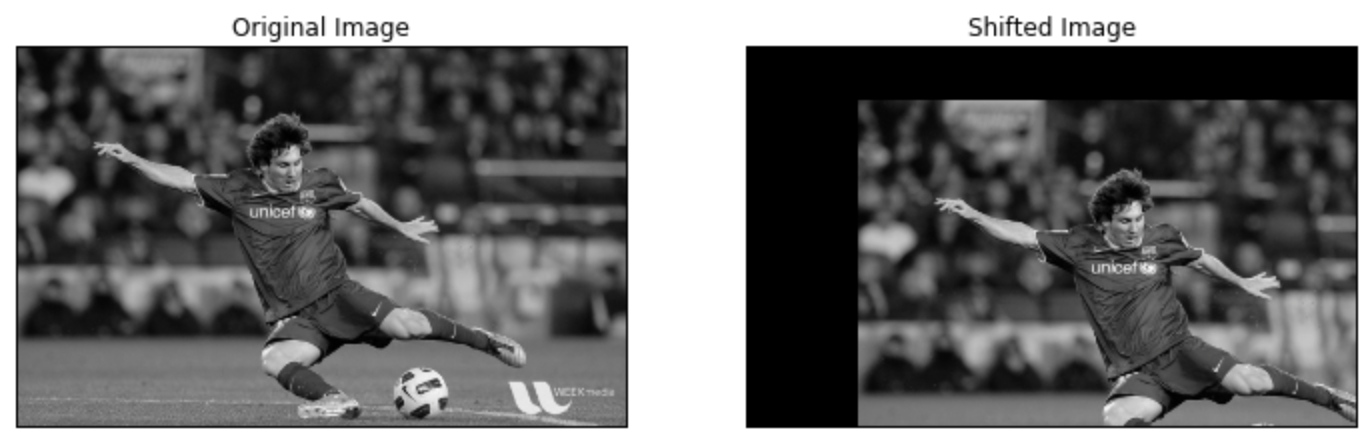
3.2.2 平移

平移是对象位置的偏移。如果你知道在((x, y))方向上的偏移量，记为((t_x, t_y))，你可以创建如下的变换矩阵：

[M = left[egin{array}{l}1 quad 0 quad t_x \ 0 quad 1 quad t_y end{array} ight] ]

你可以将矩阵构建为数据类型为np.float32的Numpy数组，并将其传递给cv2.warpAffine()函数。下面的例子实现(100, 50)的平移：

import cv2
import numpy as np

img = cv2.imread('messi5.jpg', 0)
rows, cols = img.shape

M = np.float32([[1, 0, 100], [0, 1, 50]])
dst = cv2.warpAffine(img, M, (cols, rows))

cv2.imshow('img', dst)
cv2.waitKey(0)
cv2.destroyAllWindows()

import matplotlib.pyplot as plt
%matplotlib inline

# plt.rcParams['figure.figsize'] = (12, 9)
# plt.subplot(1, 2, 1)
# plt.imshow(img, 'gray'), plt.title("Original Image"), plt.xticks([]), plt.yticks([])
# plt.subplot(1, 2, 2)
# plt.imshow(dst, 'gray'), plt.title("Shifted Image"), plt.xticks([]), plt.yticks([])

警告：
cv2.warpAffine()函数的第三个参数是输出图像的大小，表现形式为(width, height)，记住width = 列的数量， height = 行的数量。

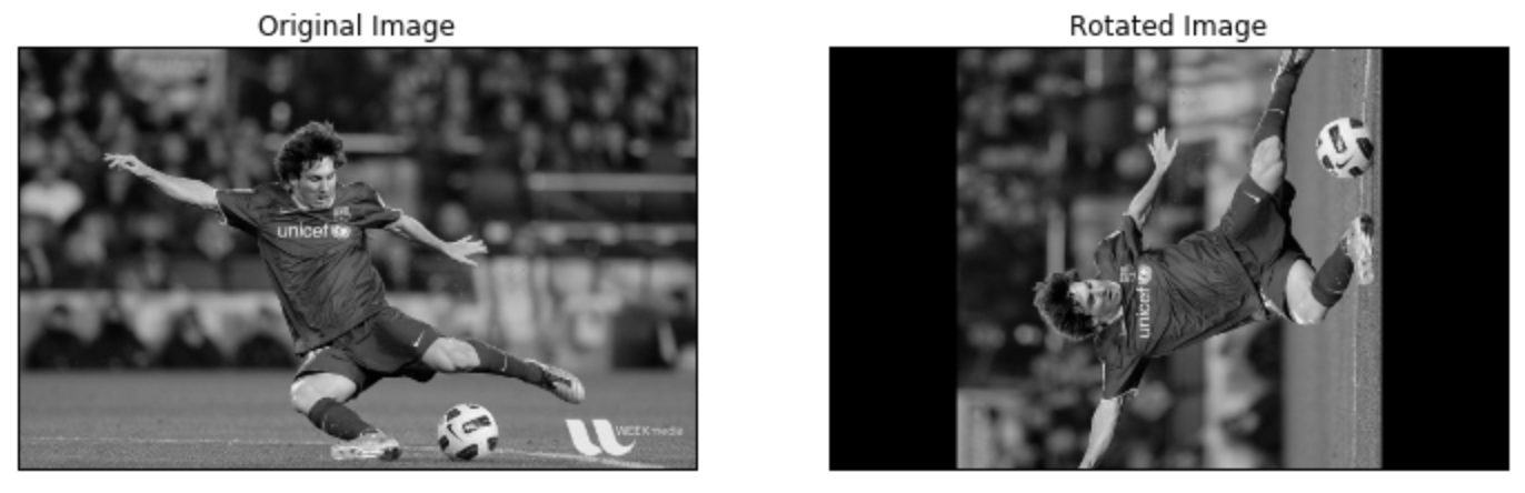
3.2.3 旋转

图像旋转( heta)度角由如下的变换矩阵完成：

[M = left[egin{array}{c} cos heta quad -sin heta \ sin heta quad cos heta end{array} ight] ]

但是OpenCV提供了扩展的旋转，你可以调整旋转中心使之在你喜欢的任何地方旋转。修改后的变换矩阵如下：

[M = egin{bmatrix} alpha quad eta quad （1-alpha)cdot ext{center.x} - eta cdot ext{center.y} \ -eta quad alpha quad eta cdot ext{center.x} + (1-alpha) cdot ext{center.y} end{bmatrix} ]

这里：

[alpha = scale cdot cos heta ]

[eta = scale cdot sin heta ]

为了找到这个变换矩阵，OpenCV提供函数cv2.getRotationMatrix2D(). 下面的例子展示了图像关于中心旋转90度，没有任何伸缩。

img = cv2.imread('messi5.jpg', 0)
rows, cols = img.shape

M = cv2.getRotationMatrix2D((cols/2, rows/2), 90, 1)
dst = cv2.warpAffine(img, M, (cols, rows))

注意：getRotationMatrix2D(center, angle, scale)
center: Center of the rotation in the source image.
angle: Rotation angle in degrees. Positive values mean counter-clockwise rotation (the coordinate origin is assumed to be the top-left corner).
scale: Isotropic scale factor.

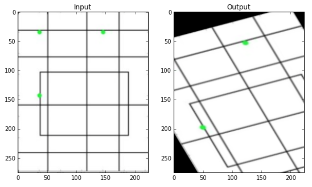
3.2.4 仿射变换

在仿射变换当中，原始图像中的平行线在输出图像中仍然是平行的。如果要找到变换矩阵，我们需要输入图像中的三个点和它们在输出图像的对应点。cv2.getAffineTransform()会创建2X3矩阵，然后传递给函数cv2.warpAffine().

查看下面的例子，并且观察我选择的点（用绿色标记）：

img = cv2.imread('drawing.png')
rows, cols, ch = img.shape

pts1 = np.float32([[50, 50], [200, 50], [50, 200]])
pts2 = np.float32([[10, 100], [200, 50], [100, 250]])

M = cv2.getAffineTransform(pts1, pts2)

dst = cv2.warpAffine(img, M, (cols, rows))

plt.rcParams['figure.figsize'] = (9, 6)
plt.subplot(121), plt.imshow(img), plt.title('Input')
plt.subplot(122), plt.imshow(dst), plt.title('Output')
plt.show()

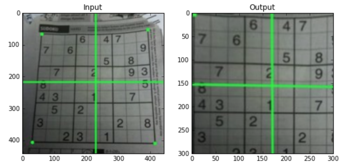
3.2.5 透视变换

对于透视变换，你需要一个3X3的变换矩阵。变换之后直线仍然是直线。如果要找到这个变换矩阵，需要输入图像的4个点和输出图像的对应点。在这4个点中，其中任何三个不能共线性。可以用函数cv2.getPerspectiveTransform()来找到变换矩阵，然后将找到的3X3变换矩阵带入到cv2.warpPerspective()函数。

代码如下：

img = cv2.imread('sudokusmall.png')
rows, cols, ch = img.shape

pts1 = np.float32([[56, 65], [368, 52], [28, 387], [389, 390]])
pts2 = np.float32([[0, 0], [300, 0], [0, 300], [300, 300]])

M = cv2.getPerspectiveTransform(pts1, pts2)

dst = cv2.warpPerspective(img, M, (300, 300))

plt.rcParams['figure.figsize'] = (9, 6)
plt.subplot(121), plt.imshow(img), plt.title('Input')
plt.subplot(122), plt.imshow(dst), plt.title('Output')
plt.show()

3.3 附加资源

“Computer Vision: Algorithms and Applications”, Richard Szeliski