Connection Management xAPP for O-RAN RIC: A Graph Neural Network and Reinforcement Learning Approach 论文解读
Abstract
Connection management is an important problem for any wireless network to ensure smooth and well-balanced operation throughout. Traditional methods for connection management (specifically user-cell association) consider sub-optimal and greedy solutions such as connection of each user to a cell with maximum receive power. However, network performance can be improved by leveraging machine learning (ML) and artificial intelligence (AI) based solutions. The next generation software defined 5G networks defined by the Open Radio Access Network (O-RAN) alliance facilitates the inclusion of ML/AI based solutions for various network problems. In this paper, we consider intelligent connection management based on the O-RAN network architecture to optimize user association and load balancing in the network. We formulate connection management as a combinatorial graph optimization problem. We propose a deep reinforcement learning (DRL) solution that uses the underlying graph to learn the weights of the graph neural networks (GNN) for optimal user-cell association. We consider three candidate objective functions: sum user throughput, cell coverage, and load balancing. Our results show up to 10% gain in throughput, 45-140% gain cell coverage, 20-45% gain in load balancing depending on network deployment configurations compared to baseline greedy techniques. Index Terms—Open Radio Access Networks, RAN Intelligent Controller, Graph Neural Networks, Deep Reinforcement learning, Connection Management, xAPP.
连接管理对于任何无线网络来说,都是确保始终流畅和均衡运行的一个重要问题。用于连接管理(特别是用户-小区关联)的传统方法考虑次优和贪婪的解决方案,例如将每个用户连接到具有最大接收功率的小区。但是,可以通过利用基于机器学习 (ML) 和人工智能 (AI) 的解决方案来提高网络性能。由开放无线电接入网络 (O-RAN) 联盟定义的下一代软件定义的 5G 网络有助于包含针对各种网络问题的基于 ML/AI 的解决方案。在本文中,我们考虑基于 O-RAN 网络架构的智能连接管理来优化网络中的用户关联和负载平衡。我们将连接管理制定为组合图优化问题。我们提出了一种深度强化学习 (DRL) 解决方案,该解决方案使用底层图来学习图神经网络 (GNN) 的权重,以获得最佳的用户-细胞关联。我们考虑三个候选目标函数:总用户吞吐量、小区覆盖和负载平衡。我们的结果表明,与基线贪婪技术相比,根据网络部署配置,吞吐量提高了 10%,小区覆盖率提高了 45-140%,负载平衡提高了 20-45%。索引词——开放无线电接入网络、RAN 智能控制器、图神经网络、深度强化学习、连接管理、xAPP
I. INTRODUCTION
Wireless communications systems, both cellular and noncellular have been evolving for several decades. We are now at the advent of fifth generation (5G) cellular wireless networks which is considered as the cellular standard to enable emerging vertical applications such as industrial internet of things, extended reality, and autonomous systems [1]. These systems impose stringent communication and computation requirements on the infrastructure serving them to deliver seamless, real-time experiences to users [2]. Traditionally, macro base stations provide cellular radio connectivity for devices which has issues such as coverage holes, call drops, jitter, high latency, and video buffering delays. To address these connectivity issues, the radio access network (RAN) needs to be brought closer to the end users. This can be achieved through network densification by deploying small cells. The target of this paper is to design and develop a scalable data-driven connection management of dense wireless links [3].

Fig. 1. ORAN architecture with distributed controllers located at CU and DU/RU, and intelligence controller RIC
A. O-RAN architecture
Typically, front-end and back-end device vendors and carriers collaborate closely to ensure compatibility. The flip-side of such a working model is that it becomes quite difficult to plug-and-play with other devices and this can hamper innovation. To combat this and to promote openness and interoperability at every level, 3rd Generation Partnership Project (3GPP) introduced RAN dis-aggregation. In parallel, several key players such as carriers, device manufacturers, academic institutions, etc., interested in the wireless domain have formed the Open Radio Access Network (O-RAN) alliance in 2018 [4]. The network architecture proposed by the O-RAN alliance is the building block for designing virtualized RAN on programmable hardware with radio access control powered by artificial intelligence (AI). The main contributions of the O-RAN architecture is a) the functionality split of central unit (CU), distributed unit (DU) and radio unit (RU), b) standardized interfaces between various units, and c) RAN intelligent controller (RIC). The CU is the central controller of the network and can serve multiple DUs and RUs which are connected through fiber links. A DU controls the radio resources, such as time and frequency bands, locally in real time. Hence, in the O-RAN architecture, the network management is hierarchical with a mix of central and distributed controllers located at CU and DUs, respectively. Another highlight of O-RAN architecture is the introduction of a RIC that leverages AI techniques to embed intelligence in every layer of the O-RAN architecture. More architectural details of ORAN are shown in Figure 1.
B. Connection Management
When a user equipment (UE) tries to connect to a network, a network entity has the functionality to provide initial access by connecting the UE to a cell. Similarly, when a UE moves it needs to keep its connection to the network for smooth operation. These functionalities are called connection management [5]. In addition to managing initial access and mobility, connection management solutions can also be programmed to achieve optimal load distribution. Traditionally, a UE triggers a handover request based on wireless channel quality measurements. The handover request is then processed by the CU. Connection management in existing solutions is performed using a UE-centric approach rather than a context-aware, network-level global approach. One of the common UE-centric techniques is received signal reference power (RSRP) based cell-UE association. When a UE moves away from a serving cell, the RSRP from the serving cell will degrade with time while its RSRP with a target cell will increase as it gets closer to it. Therefore, a simple UE-centric maximum RSRP selection approach [5] can be switching to a new cell when RSRP from the target cell is stronger than the current serving cell.
While this greedy approach is simple and effective, it does not take into consideration the network status (local and global). One of the main disadvantage of the greedy approach is the lack of load balancing – a cell can be heavily loaded/congested while other neighboring cells are underutilized, specially with non-uniform user/traffic distribution. However, O-RAN architecture provides the possibility of a more global RAN automation by leveraging machine learning (ML)-solutions in the RIC.
In ML-based optimization framework, dynamic particle swarm optimization is used to improve quality of experience of UEs for connection management in [6]. In [7], a visual-dataassisted handover optimization is considered by using neural networks. A more proactive approach by predicting obstacles to associate UEs to new cells before link disconnection is proposed in [8]. In a more distributed learning framework, authors in [9] investigate UE throughput maximization using multi-agent reinforcement learning which considers independent handover decisions based on local channel measurements. Similarly, [10] studies the same problem using deep deterministic reinforcement learning algorithm to solve the resulting non-convex optimization problem. The above machine learning algorithms do not utilize structure of wireless networks for the design of neural network architecture, and hence, may have performance loss from wireless network dynamics.
In this paper, we consider an AI-based framework for loadaware connection management which incorporates structure of wireless networks into the neural network architecture. Specifically, we focus on the problem of handover management using graph neural networks (GNN) and reinforcement rearning (RL) as our main tools. To achieve intelligent and proactive connection management, we abstract the O-RAN network as a graph, in which cells and UEs are represented by nodes and the quality of the wireless links are given by the edge weights. To capture the load-awareness, edge and node labels reflecting features, such as instantaneous load conditions, channel quality, average UE rates, etc. are considered and the proposed joint GNN-RL framework is applied to enable intelligent user handover decisions.
II. SYSTEM MODEL
In this paper, we consider an O-RAN network consisting of N cells (we assume that every RU represents a cell) and M UEs as a graph G = (V, E). The set of cell nodes are
 V cl = {v cl 0 , ..., vcl N−1 }
and the set of UE nodes are
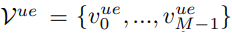 V ue = {v ue 0 , ..., vue M−1 }
with the set of all nodes in the network given by
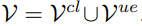 V = V cl∪Vue.
The edges
 E ue = {ev cl i ,vue j |v cl i ∈ Vcl, vue j ∈ V ue}
of G are wireless links between UEs and cells.
Although all cells are directly connected to a RIC in a tree structure, we consider virtual edges between cells (RU) to convey information about their UE connectivity and local graph structure.
The virtual edges
 E cl = {evi cl ,vcl j |v cl i , vcl j ∈ Vcl}
between two cells can be defined according to the Euclidean distance such that there is a link between two cells if the Euclidean distance between them is smaller than dmax (this is just one way to define the edges). We denote the set of UE nodes connected to a specific cell,
 vi cl, as C(v cl i) = {v ue j |ev cl i ,vue j ∈ Eue , ∀j}.
An example O-RAN network abstraction is given in Figure 2. As shown in the figure, the cell-UE connections are depicted as shaded clustering around cells, and cell-cell virtual connection graph is decided according to the Euclidean distance.
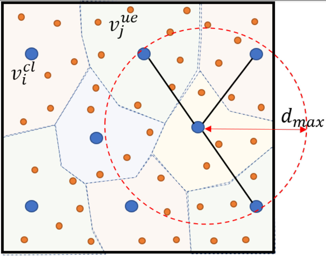
Fig. 2. An example network abstraction as a graph: blue circles are cells and orange circles are UE nodes.
The links between UEs and cells are dynamic and they depend on the mobility of the UEs. In communication theory, the channel capacity quantifies the highest information rate that can be sent reliably (with a small probability of error). A rough estimate of the single-input single-output channel capacity between base station and user device with additive white Gaussian noise (AWGN) at the receiver is given by

where N0 is the noise power and
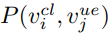 P(v cl i , vue j) is RSRP at
  v ue j from cell
  v cl i .
The above estimate is more accurate if we assume that the interference from neighboring cells is negligible and links are beamformed (especially for mmWave). We also disregard the interference from non-assigned nodes since mmWave frequency narrow beams are known to be powerlimited rather than being interference-limited. We assume that each UE measures RSRPs from close-by cells and reports them to the RIC. Then, the RIC decides on the connectivity graph between cells and UEs according to a desired network performance measure. We consider the following performance measures at the network:
• Sum throughput: Given a graph  , the network throughput is defined as a total data rate it can deliver to the UEs in the network. The throughput is computed as follows:

Here, we consider equal resource allocation between UEs connected to the same cell
• Coverage: UEs can be classified as cell-centric or celledge depending on the data rate they get. A user is considered as cell-edge if its rate is below a chosen threshold. In general, this threshold value is chosen to be the 5th percentile of the all UE rates in the network and is the coverage of the network. Higher cell-edge user rate improves network coverage and reduces coverage holes.

where 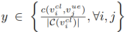
 and F(·) is cumulative distribution function (CDF).
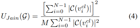
• Load balancing: In communication networks, various fairness metric are considered to ensure equitable allocation of resources [11]. In this work, we consider Jain’s index to quantitatively measure fair resource allocation between users. The Jain’s index is defined as,
In our optimization problem, we aim to find the optimal graph G∗ leading to the best UE and cell association such that a combination of the above performance measures is maximized. The optimal network topology/graph G∗ is given by:
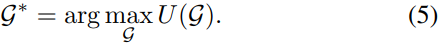
where  U(G) can be a weighted combination of performance measures defined above.
III. GRAPH NEURAL
NETWORKS Graph Neural Networks are a framework to capture the dependence of nodes in graphs via message passing between the nodes. Unlike deep neural networks, a GNN directly operates on a graph to represent information from its neighborhood with arbitrary hops. This makes GNN an apt tool to use for wireless networks which have complex features that cannot be captured in a closed form. In this paper, we consider GNNbased approach by incorporating cell-UE relationship between nodes as well as channel capacities over the edgess.
For a given network with a set of N cells and M UEs, we define two adjacency matrices: Acl ∈ {0, 1}N×N for the graph between cells and Aue ∈ {0, 1}N×M for the graph between UEs and cells, as follows:

We consider a L-layer GNN that computes on the graph. We define the initial nodal features of the cells and UEs as (X (0) cl,1 , X (0) cl,2 ) and X (0) ue , respectively. The initial nodal features are functions of reported channel capacities and data rates at the cell and UE. We define C ∈ R N×M as channel capacity matrix with elements c(vcli , vuej ), and R ∈ RN×M as user rate matrix with elements c(v cli ,vuej ) /|C(vcli )| for a given cell-UE connectivity graph. We calculate input features as follows:

where [·||·] is vector concatenation operator and 1M and 1N are all-ones vector of size M and N, respectively. All the above latent features capture either node sum rate or sum rates of neighboring cells or channel capacity/data rate in the case of UEs. These are selected as the features since they capture the information relevant to making connectivity decisions.
At every layer, the GNN computes a d-dimensional latent feature vector for each node vcli , vuej ∈ V in the graph G. The latent feature calculation at layer l can be written as follows:

In the above equations, W(0) k ∈ R 2×d and W(l) k ∈ R d×d (for l > 0), k = 1, 2, 3, are neural network weights, l is the layer index of GNN, and σ(·) is a non-linear activation function. Note that H (l) cl and H (l) ue are auxiliary matrices which represent sum of hidden features of cell-cell and cell-UE connectivity graphs. Equations (13)-(15) represent a spatial diffusion convolution neural network [12]. The L-layer GNN essentially repeats the above calculation for l = 0, 1, .., L − 1. Through this, features of the nodes are propagated to other nodes and will get aggregated at distant nodes. This way each node’s feature will contain information about its L-hop neighbors, as the embedding is carried out L-times. We combine the feature vectors at the last layer of GNN to get a scalar-valued score for G. We sum the output layer of GNN over cells, H (L−1) cl , which makes the score calculation invariant to permutation over nodes, before passing it to single layer fully connected neural network. We get network score of the graph G as follows:

where 1TN is the all-ones vector of size N, W4 ∈ Rd×d is the fully connected neural network weight matrix, and w5 ∈ Rd×1 is the vector to combine neural network output, linearly. Once the GNN computations are complete, the score of G, Q(G), will be used to select the best connection graph among subset of feasible graphs. The procedure to learn the optimal weights W(l)k , ∀k, l, and w5 is described in the next section.
IV. DEEP Q-LEARNING ALGORITHM
We propose a deep Q-learning approach [13], in which a Q-function is learned from cell and UE deployment instances and the corresponding reward we get from the network environment. The advantage of the proposed GNN formulation as the neural network for the Q-function is that GNN is scalable to different graph sizes and can capture local network features with variable numbers of cells and UEs. To make the best selection for UE connectivity, we need to learn the right Q-function. As the Q-function is captured through the GNN, this translates to learning the parameters of the GNN which we do through sequential addition of new cell-UE connections to partially connected graph. The state, action, and reward in the deep RL framework are defined as follows:
• State st: The state is defined as the current graph Gt containing the cells and connected UEs at iteration t as well as input features of nodes X(0)cl and X(0)ue . The start state can be considered as partially connected network with connected and unconnected UEs. The terminal state sT is achieved when all the UEs in the network are connected.
• Action at: The action at = Gt ∪ evcli ,vuej at step t is to connect an unconnected UE to one of the cells.
• Reward r(st, at): The reward at state st after selecting action at is

i.e., the reward is defined as the change in the network utility function after connecting a new UE. In section V-B, we provide various reward functions for the performance measures given in Section II.
• Policy π(at|st): We use a deterministic greedy policy, i.e., π(at|st) = arg maxat Q(st, at) with ε-greedy exploration during training. Here, Q(st, at) is defined in Eq. (16) with Gt = st ∪ evcli ,vuej
Algorithm 1 describes the proposed deep Q-network (DQN) approach. First, the parameters are initialized and defined for each deployment. In each step t, one UE at = evcli ,vuej is connected by following the ε-greedy policy π(at|st), with ε being the exploration rate. Here, the number of steps T is given by the termination state sT . The graph Gt is updated, so that the next step st+1 is obtained. The new nodal input features X(0)cl and X(0)ue are calculated every time the graph is updated,
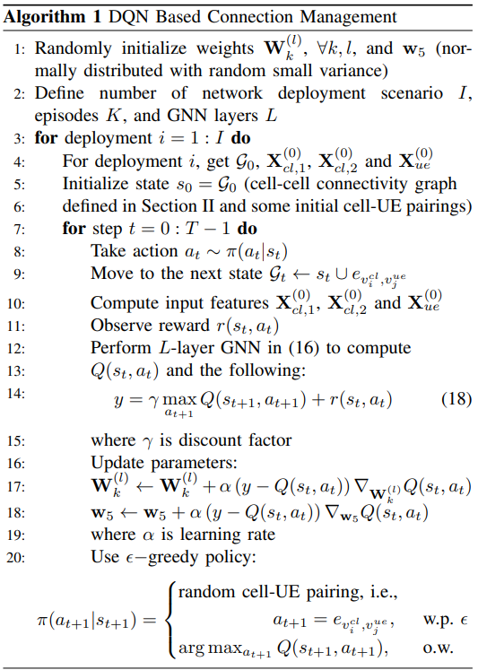
and the reward r(st, at) is calculated for each selected action. The L-layer GNN computation provides the score for each state and action pair.
Then, to learn the neural network weights W(l)k , ∀k, l, and w5, Q-learning updates parameters by performing Stochastic Gradient Descent (SGD) to minimize the squared loss E{(y − Q(st, at))2 }, with y being defined in Eq. (18) and γ being the discount factor. Algorithm 1 reflects the training phase. Once the training is completed, the neural network weights are not updated and they are used directly to obtain the actions for unseen deployment instances.
V. IMPLEMENTATION AND EVALUATION
A. xApp Implementation at O-RAN RIC
O-RAN defines xApp as an application designed to run on the near real-time operation at the RIC [4]. These xApps consist of several microservices which get input data through interfaces between O-RAN RIC and RAN functionality, and provides additional functionality as output to RAN. This section mainly addresses the methods to make the xApp scalable and provides an overview on how the connection management algorithm is deployed and realized in O-RAN architecture. Even though it also works for initial access, we consider the proposed GNN-RL based connection management algorithm for handover application in which mobile users in the network request for new cell connections. We refer to the request for a new cell connection as a handover event. A UE continuously measures the RSRPs from its surrounding cells. If certain conditions are met (as defined in the 3GPP standards), the UE reports the measured RSRPs for a handover request. When the O-RAN RIC receives a handover event, the GNN-RL algorithm makes new connection decisions to balance the load of the network.
We expect that the O-RAN RIC consists of 100s of cells and 1000s of UEs. The large scale O-RAN deployment will result in a large network topology graph G and which increases the processing latency and complexity of the GNN-RL inference. We consider two solutions to reduce dimension of GNN-RL inference. First, we consider a local sub-graph of the O-RAN network around a handover requested UE. This local sub-graph includes only those cells whose RSRP is reported by UE that has issued the handover request and the L−hop neighbors of the these cells in the virtual cell-cell connection graph as defined in Section II. Here, L is the number of layer of GNN as defined in Section III. Second, we classify each UE in the network as either a cell-edge or a cell-center UE. The cell-edge UEs are defined as the UEs that are close to the boundary of the cell’s coverage as shown in Figure 2. We mark the UE as a cell edge UE if the difference between the strongest and the second strongest RSRP measurements is less than a given threshold e.g. 3dB. The remaining UEs are marked as cellcenter UEs since their strongest RSRP measurement is larger than their other measurements, and hence, does not need a new cell connection. Therefore, the initial connectivity graph G0 of the GNN-RL includes an edge between a cell and a UE if it is a cell-center UE. We refer to the set of cell-edge UEs in the sub-graph as reshuffled UEs. The solution proposed above enables us to reduce the total action space of the RL algorithm by reducing the number of reshuffled UEs, T, in the initial connectivity graph G0 in Algorithm 1.
B. Training
To showcase the benefits of the proposed GNN-RL algorithm in various use cases and applications, we train the GNN with two different reward functions described below. Then, we evaluate the performance with metrics given in Section II. For data intensive applications where maximizing throughput is more important, we consider the sum throughput utility function given in Eq. (2) to calculate reward as follows:

For applications that prioritize fairness among users, we consider the following reward function which is weighted sum of improvement in total network throughput and the smallest user rate at each cell in the network (captured by the second term in the equation below):

Note that the last term in the above equation tries to maximize the minimum user rate. Increasing the minimum user rate helps to maximize the network coverage given in Eq. (3) and fairness given in Eq. (4) by closing the rate gap between users.
We consider uniformly distributed cells and UEs in a hexagonal network area. The consideration of random deployment is useful to generalize inference performance to many real world cases such as varying city block sizes, rural or urban areas, hot spots at stadiums and concerts. We follow 3GPP network settings and channel models [14]. The cell transmit power is 33 dBm. The carrier frequency of channel is 30GHz with the large scale channel parameters and 100MHz channel bandwidth [15]. In the network, each UE measures the RSRP from its current serving cell and its three closest cells, and reports the measurements back to the O-RAN RIC.
For training the GNN, we collect 1000 deployment scenarios with 6 cells and 50 UEs. We set the diameter of hexagonal area to 500m and select 6 cells in the area which corresponds to about 37 cells per km2 . For the GNN architecture, we have L = 2 layers, and d = 8 dimensions per layer. For the reinforcement learning algorithm, we consider exploration rate ξ = 0.1, learning rate α = 0.1 and discount factor γ = 1. Additionally, we consider experience buffer of size 8 to reduce the impact of correlation between consecutive UE association
C. Numerical Results
We compare GNN-RL solution with the maximum RSRP benchmark algorithm. In the benchmark algorithm, each UE is associated with a cell from which it receives the strongest RSRP. As discussed in Section II, the benchmark algorithm is UE-centric and greedy. To show the scalability and robustness benefits of the GNN-RL approach, we collect 50 different deployment scenarios for different number of cells and UEs and network densities.
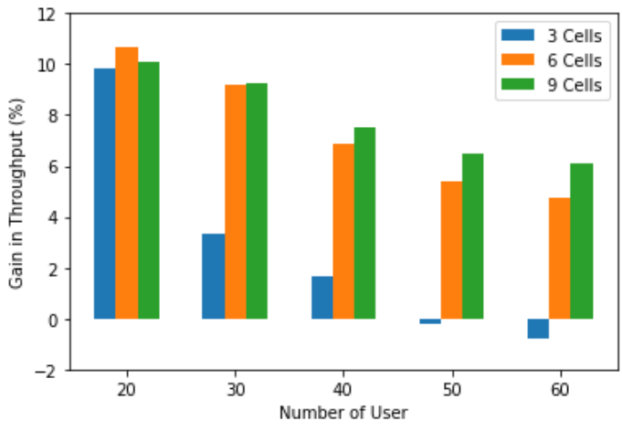
Fig. 3. Throughput gain of GNN-RL with various network sizes
In Fig. 3, we depict the relative gain of throughput defined in (2) of GNN-RL approach over the maximum RSRP algorithm. In this case, the GNN weights are obtained using reward function given in Eq. (19). As shown in the figure, we observe up to 10% gain when the number of UEs is small and as the number of users increases the gain drops. This is expected because when the number of users is small, each user gets larger share from the network, and a connection decision made by the GNN-RL approach has more impact on the performance. On the other hand, as the network size scales up with the number of cells while keeping diameter of hexagonal network area the same, we also observe more gain in performance which shows scalability and robustness benefits of the GNN architecture.
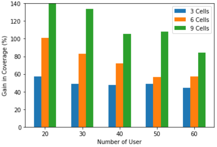
Fig. 4. Coverage gain of GNN-RL with various network sizes
In Fig. 4 and 5, we show the relative gain of coverage and load balancing defined in Eq (3) and (4), respectively, of GNNRL approach over the maximum RSRP algorithm. Here, we train the GNN with the reward function given in Eq. (20). We observe similar trends as in Fig. 3. However, the relative gains in coverage and load balancing is much larger than the throughput gain which shows the importance of GNN based solution for handover applications.
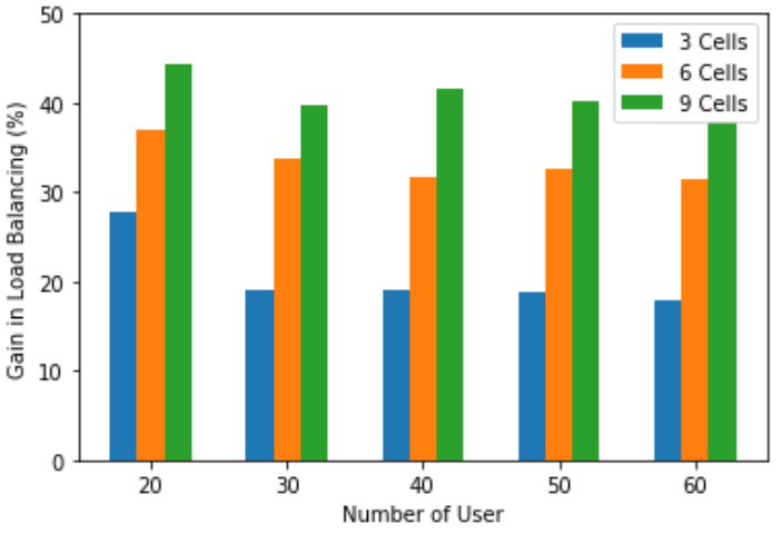
Fig. 5. Load balancing gain of GNN-RL with various network sizes
Fig. 6 shows the benefit of GNN-RL approach to varying network densities in terms of number of cell per km2 while keeping the average number of UEs per cell the same. As argued before, we train the neural network only for the scenario with 37 cells per km2 network density and use trained model to test different network densities. We observe more gain in coverage as network gets denser because when network is dense, cell edge users have multiple good cell selection options and GNN-RL approach makes better decisions compared to greedy cell selection. Additionally, high performance gains in different network densities show that the GNN-RL approach is robust to any network deployment scenario.

Fig. 6. Gain of GNN-RL with various network densities
VI. CONCLUSION
In this paper, we introduce connection management for O-RAN RIC architecture based on GNN and deep RL. The proposed approach considers the graph structure of the O-RAN architecture as the building block of neural network architecture and use RL to learn the parameters of the algorithm. The main advantage of the algorithm is that it can consider local network features to make better decisions to balance network traffic load while network throughput is also maximized. We also demonstrate that the proposed approach is scalable and robust against different network scenarios, and outperforms the existing RSRP based algorithm.
REF:
Connection Management xAPP for O-RAN RIC: A Graph Neural Network and Reinforcement Learning Approach