python 数据分析-- 实战1（收入预测分析）

说明：

本文用途只做学习记录：

• 参考书籍：从零开始学Python数据分析与挖掘／刘顺祥著．—北京：清华大学出版社，2018
• 数据下载：链接：https://pan.baidu.com/s/1VhnNfUNgNLICIFRyrlteOg提取码：m1dl

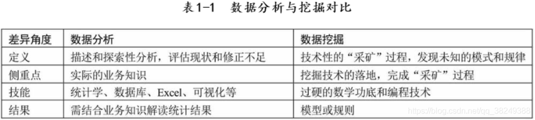
首先看一下刘老师介绍的数据分析和数据挖掘的区别：

1. 预览数据集，明确分析目的

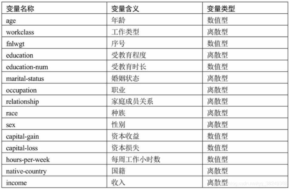
通过Excel工具打开income文件，可发现该数据集一共有 32 561条样本数据，共有15个数据变量，其中9个离散型变量，6个数值型变量。数据项主要包括：年龄，工作类型，受教育程度，收入等，具体可见下面两个图：

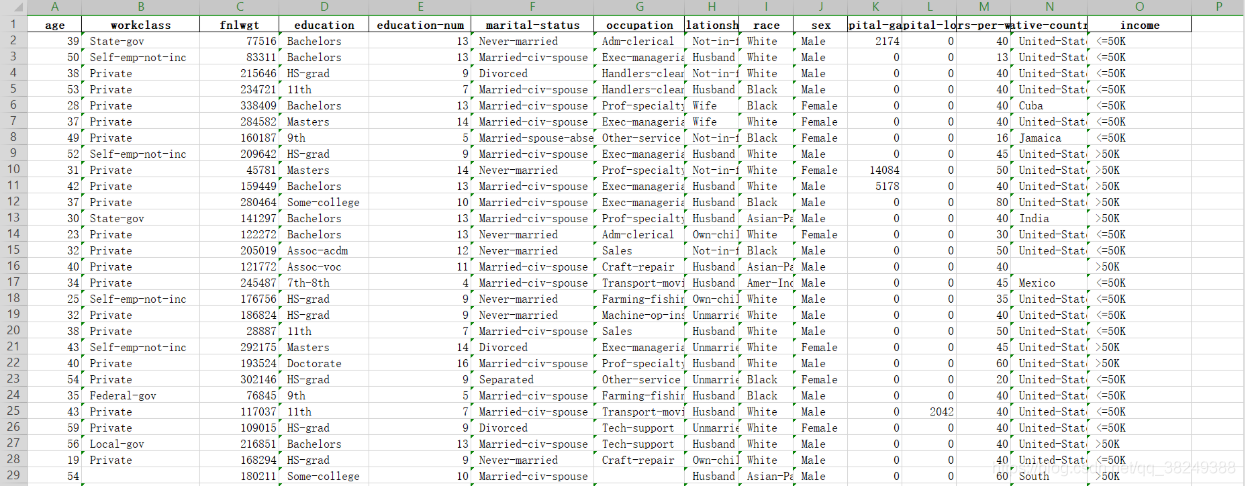
拿到上面的数据集，我们观察这些数据都有什么用，想一想这张数据表中income比较特殊，有分析价值，其他变量的不同会对income产生一定的影响。

实验目的：因此，基于上面的数据集，需要预测居民的年收入是否会超过5万美元？

2. 导入数据集，预处理数据

在jupyter notebook中导入相应包，读取数据，进行预处理。在上述数据集中，有许多变量都是离散型的，如受教育程度、婚姻状态、职业、性别等。通常数据拿到手后，都需要对其进行清洗，例如检查数据中是否存在重复观测、缺失值、异常值等，而且，如果建模的话，还需要对字符型的离散变量做相应的重编码。

import numpy as np
import pandas as pd 
import seaborn as sns

# 下载的数据集存放的路径：
income = pd.read_excel(r'E:Data1income.xlsx')

# 查看数据集是否存在缺失
income.apply(lambda x:np.sum(x.isnull()))

age                  0
workclass         1836
fnlwgt               0
education            0
education-num        0
marital-status       0
occupation        1843
relationship         0
race                 0
sex                  0
capital-gain         0
capital-loss         0
hours-per-week       0
native-country     583
income               0
dtype: int64

从上面的结果可以发现，居民的收入数据集中有3个变量存在数值缺失，分别是居民的工作类型（离散型）缺1836、职业（离散型）缺1843和国籍（离散型）缺583。缺失值的存在一般都会影响分析或建模的结果，所以需要对缺失数值做相应的处理。
缺失值的处理一般采用三种方法：

• 1.删除法，缺失的数据较少时适用；
• 2.替换法，用常数替换缺失变量，离散变量用众数，数值变量用均值或中位数；
• 3.插补法：用未缺失的预测该缺失变量。

根据上述方法，三个缺失变量都为离散型，可用众数替换。pandas中fillna()方法，能够使用指定的方法填充NA/NaN值。
函数形式：
fillna(value=None, method=None, axis=None, inplace=False, limit=None, downcast=None, **kwargs)
参数：

• value：用于填充的空值的值。（该处为字典）

• method： {'backfill', 'bfill', 'pad', 'ffill', None}, default None。定义了填充空值的方法， pad/ffill表示用前面行/列的值，填充当前行/列的空值， backfill / bfill表示用后面行/列的值，填充当前行/列的空值。

• axis：轴。0或'index'，表示按行删除；1或'columns'，表示按列删除。

• inplace：是否原地替换。布尔值，默认为False。如果为True，则在原DataFrame上进行操作，返回值为None。

• limit：int，default None。如果method被指定，对于连续的空值，这段连续区域，最多填充前 limit 个空值（如果存在多段连续区域，每段最多填充前 limit 个空值）。如果method未被指定， 在该axis下，最多填充前 limit 个空值（不论空值连续区间是否间断）

• downcast：dict, default is None，字典中的项，为类型向下转换规则。或者为字符串“infer”，此时会在合适的等价类型之间进行向下转换，比如float64 to int64 if possible。

# 缺失值处理，采用众数替换法（mode（）方法取众数）
income.fillna(value={'workclass':income['workclass'].mode()[0],
                     'ouccupation':income['occupation'].mode()[0],
                     'native-country':income['native-country'].mode()[0]},
              inplace = True)

3. 探索数据背后的特征

对缺失值采用了替换处理的方法，接下来对居民收入数据集做简单的探索性分析，目的是了解数据背后的特征如数据的集中趋势、离散趋势、数据形状和变量间的关系等。首先，需要知道每个变量的基本统计值，如均值、中位数、众数等，只有了解了所需处理的数据特征，才能做到“心中有数”。

3.1 数值型变量统计描述

# 3.1 数值型变量统计描述
income.describe()

	age	fnlwgt	education-num	capital-gain	capital-loss	hours-per-week
count	32561.000000	3.256100e+04	32561.000000	32561.000000	32561.000000	32561.000000
mean	38.581647	1.897784e+05	10.080679	1077.648844	87.303830	40.437456
std	13.640433	1.055500e+05	2.572720	7385.292085	402.960219	12.347429
min	17.000000	1.228500e+04	1.000000	0.000000	0.000000	1.000000
25%	28.000000	1.178270e+05	9.000000	0.000000	0.000000	40.000000
50%	37.000000	1.783560e+05	10.000000	0.000000	0.000000	40.000000
75%	48.000000	2.370510e+05	12.000000	0.000000	0.000000	45.000000
max	90.000000	1.484705e+06	16.000000	99999.000000	4356.000000	99.000000

上面的结果描述了有关数值型变量的简单统计值，包括非缺失观测的个数（count）、平均值（mean）、标准差（std）、最小值（min）、下四分位数（25%）、中位数（50%）、上四分位数（75%）和最大值（max）。

3.2 离散型变量统计描述

# 2. 离散型变量统计描述
income.describe(include= ['object'])

	workclass	education	marital-status	occupation	relationship	race	sex	native-country	income
count	32561	32561	32561	30718	32561	32561	32561	32561	32561
unique	8	16	7	14	6	5	2	41	2
top	Private	HS-grad	Married-civ-spouse	Prof-specialty	Husband	White	Male	United-States	<=50K
freq	24532	10501	14976	4140	13193	27816	21790	29753	24720

上面为离散变量的统计值，包含每个变量非缺失观测的数量（count）、不同离散值的个数（unique）、出现频次最高的离散值（top）和最高频次数（freq）。以受教育水平变量为例，一共有16种不同的教育水平；3万多居民中，高中毕业的学历是出现最多的；并且一共有10 501名。

3 .3 了解数据的分布形状

为了了解数据的分布形状（如偏度、峰度等）可以通过可视化的方法进行展现。

#以被调查居民的年龄和每周工作小时数为例，绘制各自的分布形状图：
import matplotlib.pyplot as plt

# 设置绘图风格
plt.style.use('ggplot')

# 设置多图形的组合
fig, axes = plt.subplots(3,1)

# 绘制不同收入水平下的年龄核密度图，观察连续型变量的分布情况
income.age[income.income == ' <=50K'].plot(kind = 'kde', label = '<=50K', ax = axes[0], legend = True, linestyle = '-')
income.age[income.income == ' >50K'].plot(kind = 'kde', label = '>50K', ax = axes[0], legend = True, linestyle = '--')

# 绘制不同收入水平下的周工作小时核密度图
income['hours-per-week'][income.income == ' <=50K'].plot(kind = 'kde', label = '<=50K', ax = axes[1], legend = True, linestyle = '-')
income['hours-per-week'][income.income == ' >50K'].plot(kind = 'kde', label = '>50K', ax = axes[1], legend = True, linestyle = '--')


# 绘制不同收入水平下的受教育时长核密度图
income['education-num'][income.income == ' <=50K'].plot(kind = 'kde', label = '<=50K', ax = axes[2], legend = True, linestyle = '-')
income['education-num'][income.income == ' >50K'].plot(kind = 'kde', label = '>50K', ax = axes[2], legend = True, linestyle = '--')

第一幅图展现的是，在不同收入水平下，年龄的核密度分布图，对于年收入超过5万美元的居民来说，他们的年龄几乎呈现正态分布，而收入低于5万美元的居民，年龄呈现右偏特征，即年龄偏大的居民人数要比年龄偏小的人数多。

第二幅图展现了不同收入水平下，周工作小时数的核密度图，很明显，两者的分布趋势非常相似，并且出现局部峰值。

第三幅图展现了不同收入水平下，教育时长的核密度图，很明显，两者的分布趋势非常相似，并且也多次出现局部峰值。
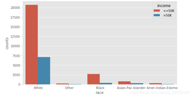
针对离散型变量，对比居民的收入水平高低在性别、种族状态、家庭关系等方面的差异，进而可以发现这些离散变量是否影响收入水平：

# 构造不同收入水平下各种族人数的数据
race = pd.DataFrame(income.groupby(by = ['race','income']).aggregate(np.size).loc[:,'age'])
#print(race)

# 重设行索引
race = race.reset_index()
#print(race)

# 变量重命名
race.rename(columns={'age':'counts'}, inplace=True)
#print(race)

# 排序
race.sort_values(by = ['race','counts'], ascending=False, inplace=True)
#print(race)

# 构造不同收入水平下各家庭关系人数的数据
relationship = pd.DataFrame(income.groupby(by = ['relationship','income']).aggregate(np.size).loc[:,'age'])
relationship = relationship.reset_index()
relationship.rename(columns={'age':'counts'}, inplace=True)
relationship.sort_values(by = ['relationship','counts'], ascending=False, inplace=True)

# 构造不同收入水平下各男女人数的数据
sex = pd.DataFrame(income.groupby(by = ['sex','income']).aggregate(np.size).loc[:,'age'])
sex = sex.reset_index()
sex.rename(columns={'age':'counts'}, inplace=True)
sex.sort_values(by = ['sex','counts'], ascending=False, inplace=True)

# 设置图框比例，并绘图
plt.figure(figsize=(9,5))
sns.barplot(x="race", y="counts", hue = 'income', data=race)
plt.show()

plt.figure(figsize=(9,5))
sns.barplot(x="relationship", y="counts", hue = 'income', data=relationship)
plt.show()

plt.figure(figsize=(9,5))
sns.barplot(x="sex", y="counts", hue = 'income', data=sex)
plt.show()

图一、反映的是相同的种族下，居民年收入水平高低的人数差异；图二、反映的是相同的家庭成员关系下，居民年收入水平高低的人数差异。但无论怎么比较，都发现一个规律，即在某一个相同的水平下（如白种人或未结婚人群中），年收入低于5万美元的人数都要比年收入高于5万美元的人数多，这个应该是抽样导致的差异（数据集中年收入低于5万和高于5万的居民比例大致在75%:25%）。图三、反映的是相同的性别下，居民收入水平高低人数的差异；其中，女性收入低于5万美元的人数比高于5万美元人数的差异比男性更严重，比例大致为90%:10%， 男性大致为70%：30%。

4. 数据建模

4.1 对离散变量重编码

由于数据集中有很多离散型变量，这些变量的值为字符串，不利于建模，因此，需要先对这些变量进行重新编码。编码的方法有很多种：

• 将字符型的值转换为整数型的值
• 哑变量处理（0-1变量）
• One-Hot热编码（类似于哑变量）
  

在本案例中，将采用“字符转数值”的方法对离散型变量进行重编码

# 离散型变量的重编码
for feature in income.columns:
    if income[feature].dtype == 'object':
        income[feature] = pd.Categorical(income[feature]).codes
income.head(10)

	age	workclass	fnlwgt	education	education-num	marital-status	occupation	relationship	race	sex	capital-gain	capital-loss	hours-per-week	native-country	income
0	39	6	77516	9	13	4	0	1	4	1	2174	0	40	38	0
1	50	5	83311	9	13	2	3	0	4	1	0	0	13	38	0
2	38	3	215646	11	9	0	5	1	4	1	0	0	40	38	0
3	53	3	234721	1	7	2	5	0	2	1	0	0	40	38	0
4	28	3	338409	9	13	2	9	5	2	0	0	0	40	4	0
5	37	3	284582	12	14	2	3	5	4	0	0	0	40	38	0
6	49	3	160187	6	5	3	7	1	2	0	0	0	16	22	0
7	52	5	209642	11	9	2	3	0	4	1	0	0	45	38	1
8	31	3	45781	12	14	4	9	1	4	0	14084	0	50	38	1
9	42	3	159449	9	13	2	3	0	4	1	5178	0	40	38	1

对字符型离散变量的重编码效果，所有的字符型变量都变成了整数型变量，接下来就基于这个处理好的数据集对收入水平income进行预测。
在原本的居民收入数据集中，关于受教育程度的有两个变量，一个是education（教育水平），另一个是education-num（受教育时长），而且这两个变量的值都是一一对应的，只不过一个是字符型，另一个是对应的数值型，如果将这两个变量都包含在模型中的话，就会产生信息的冗余；fnlwgt变量代表的是一种序号，其对收入水平的高低并没有实际意义。故为了避免冗余信息和无意义变量对模型的影响，考虑将education变量和fnlwgt变量从数据集中删除。

income.drop(['education','fnlwgt'], axis=1, inplace=True)
income.head(10)

	age	workclass	education-num	marital-status	occupation	relationship	race	sex	capital-gain	capital-loss	hours-per-week	native-country	income
0	39	6	13	4	0	1	4	1	2174	0	40	38	0
1	50	5	13	2	3	0	4	1	0	0	13	38	0
2	38	3	9	0	5	1	4	1	0	0	40	38	0
3	53	3	7	2	5	0	2	1	0	0	40	38	0
4	28	3	13	2	9	5	2	0	0	0	40	4	0
5	37	3	14	2	3	5	4	0	0	0	40	38	0
6	49	3	5	3	7	1	2	0	0	0	16	22	0
7	52	5	9	2	3	0	4	1	0	0	45	38	1
8	31	3	14	4	9	1	4	0	14084	0	50	38	1
9	42	3	13	2	3	0	4	1	5178	0	40	38	1

上面表格呈现的就是经处理“干净”的数据集，所要预测的变量就是income，该变量是二元变量，对其预测的实质就是对年收入水平的分类（一个新样本进来，通过分类模型，可以将该样本分为哪一种收入水平）。

关于分类模型有很多种：

• Logistic模型
• 决策树
• K近邻
• 朴素贝叶斯模型
• 支持向量机
• 随机森林
• 梯度提升树GBDT模型等。

本案例将对比使用K近邻和GBDT两种分类器，因为通常情况下，都会选用多个模型作为备选，通过对比才能得知哪种模型可以更好地拟合数据。

4.2 拆分数据集

接下来就进一步说明如何针对分类问题，从零开始完成建模的步骤。基于上面的“干净”数据集，需要将其拆分为两个部分，一部分用于分类器模型的构建，另一部分用于分类器模型的评估，这样做的目的是避免分类器模型过拟合或欠拟合。如果模型在训练集上表现很好，而在测试集中表现很差，则说明分类器模型属于过拟合状态；如果模型在训练过程中都不能很好地拟合数据，那说明模型属于欠拟合状态。通常情况下，会把训练集和测试集的比例分配为75%和25%。

# 导入sklearn包中的函数
from sklearn.model_selection import train_test_split

# 拆分数据
X_train, X_test, y_train, y_test = train_test_split(income.loc[:,'age':'native-country'],
                                                   income['income'],train_size = 0.75,test_size=0.25, random_state = 1234)
# print(X_train)
# print(y_train)
print("训练数据集中共有 %d 条观测"  %X_train.shape[0])
print("测试数据集中共有 %d 条测试" %X_test.shape[0])

训练数据集中共有 24420 条观测
测试数据集中共有 8141 条测试

上面的结果，运用随机抽样的方法，将数据集拆分为两部分，其中训练数据集包含24 420条样本，测试数据集包含8 141条样本，下面将运用拆分好的训练数据集开始构建K近邻和GBDT两种分类器。

4.3 搭建模型

# 导入K近邻模型的类
from sklearn.neighbors import KNeighborsClassifier
from sklearn.ensemble import GradientBoostingClassifier 

# 构件K近邻模型
kn = KNeighborsClassifier()
kn.fit(X_train,y_train)
print(kn)

#构件GBDT模型
gbdt = GradientBoostingClassifier()
gbdt.fit(X_train, y_train)
print(gbdt)

KNeighborsClassifier(algorithm='auto', leaf_size=30, metric='minkowski',
           metric_params=None, n_jobs=1, n_neighbors=5, p=2,
           weights='uniform')
GradientBoostingClassifier(criterion='friedman_mse', init=None,
              learning_rate=0.1, loss='deviance', max_depth=3,
              max_features=None, max_leaf_nodes=None,
              min_impurity_decrease=0.0, min_impurity_split=None,
              min_samples_leaf=1, min_samples_split=2,
              min_weight_fraction_leaf=0.0, n_estimators=100,
              presort='auto', random_state=None, subsample=1.0, verbose=0,
              warm_start=False)

首先，针对K近邻模型，这里直接调用sklearn子模块neighbors中的KNeighborsClassifier类，并且使用模型的默认参数，即让K近邻模型自动挑选最佳的搜寻近邻算法（algorithm='auto'）、使用欧氏距离公式计算样本间的距离（p=2）、指定未知分类样本的近邻个数为5（n_neighbors=5）而且所有近邻样本的权重都相等（weights='uniform'）。其次，针对GBDT模型，可以调用sklearn子模块ensemble中的GradientBoostingClassifier类，同样先尝试使用该模型的默认参数，即让模型的学习率（迭代步长）为0.1（learning_rate=0.1）、损失函数使用的是对数损失函数（loss='deviance'）、生成100棵基础决策树（n_estimators=100），并且每棵基础决策树的最大深度为3（max_depth=3），中间节点（非叶节点）的最小样本量为2（min_samples_split=2），叶节点的最小样本量为1（min_samples_leaf=1），每一棵树的训练都不会基于上一棵树的结果（warm_start=False）。

4.4 模型网格搜索法，探寻模型最佳参数

# K 近邻模型网格搜索法
# 导入网格搜索函数
from sklearn.grid_search import GridSearchCV
# 选择不同的参数
k_options = list(range(1,12))
parameters = {'n_neighbors':k_options}
# 搜索不同的K值
grid_kn = GridSearchCV(estimator= KNeighborsClassifier(), param_grid=parameters, cv=10, scoring='accuracy')
grid_kn.fit(X_train, y_train)
# 结果输出
grid_kn.grid_scores_, grid_kn.best_params_, grid_kn.best_score_

([mean: 0.81507, std: 0.00711, params: {'n_neighbors': 1},
  mean: 0.83882, std: 0.00696, params: {'n_neighbors': 2},
  mean: 0.83722, std: 0.00843, params: {'n_neighbors': 3},
  mean: 0.84586, std: 0.01039, params: {'n_neighbors': 4},
  mean: 0.84222, std: 0.00916, params: {'n_neighbors': 5},
  mean: 0.84713, std: 0.00900, params: {'n_neighbors': 6},
  mean: 0.84316, std: 0.00719, params: {'n_neighbors': 7},
  mean: 0.84525, std: 0.00629, params: {'n_neighbors': 8},
  mean: 0.84394, std: 0.00678, params: {'n_neighbors': 9},
  mean: 0.84570, std: 0.00534, params: {'n_neighbors': 10},
  mean: 0.84464, std: 0.00444, params: {'n_neighbors': 11}],
 {'n_neighbors': 6},
 0.8471334971334972)

GridSearchCV函数中的几个参数含义，estimator参数接受一个指定的模型，这里为K近邻模型的类；param_grid用来指定模型需要搜索的参数列表对象，这里是K近邻模型中n_neighbors参数的11种可能值；cv是指网格搜索需要经过10重交叉验证；scoring指定模型评估的度量值，这里选用的是模型预测的准确率。通过网格搜索的计算，得到三部分的结果，第一部分包含了11种K值下的平均准确率（因为做了10重交叉验证）；第二部分选择出了最佳的K值，K值为6；第三部分是当K值为6时模型的最佳平均准确率，且准确率为84.78%。

# GBDT 模型的网格搜索法
# 选择不同的参数
from sklearn.grid_search import GridSearchCV
learning_rate_options = [0.01, 0.05, 0.1]
max_depth_options = [3,5,7,9]
n_estimators_options = [100, 300, 500]

parameters = {'learning_rate':learning_rate_options,
             'max_depth':max_depth_options,
             'n_estimators':n_estimators_options}

grid_gbdt = GridSearchCV(estimator= GradientBoostingClassifier(),param_grid=parameters,cv=10,scoring='accuracy')
grid_gbdt.fit(X_train, y_train)

# 结果输出
grid_gbdt.grid_scores_,grid_gbdt.best_params_, grid_gbdt.best_score_

([mean: 0.84267, std: 0.00727, params: {'learning_rate': 0.01, 'max_depth': 3, 'n_estimators': 100},
  mean: 0.85360, std: 0.00837, params: {'learning_rate': 0.01, 'max_depth': 3, 'n_estimators': 300},
  mean: 0.85930, std: 0.00746, params: {'learning_rate': 0.01, 'max_depth': 3, 'n_estimators': 500},
  mean: 0.85213, std: 0.00821, params: {'learning_rate': 0.01, 'max_depth': 5, 'n_estimators': 100},
  mean: 0.86327, std: 0.00751, params: {'learning_rate': 0.01, 'max_depth': 5, 'n_estimators': 300},
  mean: 0.86929, std: 0.00767, params: {'learning_rate': 0.01, 'max_depth': 5, 'n_estimators': 500},
  mean: 0.85459, std: 0.00767, params: {'learning_rate': 0.01, 'max_depth': 7, 'n_estimators': 100},
  mean: 0.87076, std: 0.00920, params: {'learning_rate': 0.01, 'max_depth': 7, 'n_estimators': 300},
  mean: 0.87342, std: 0.00983, params: {'learning_rate': 0.01, 'max_depth': 7, 'n_estimators': 500},
  mean: 0.85438, std: 0.00801, params: {'learning_rate': 0.01, 'max_depth': 9, 'n_estimators': 100},
  mean: 0.86855, std: 0.00907, params: {'learning_rate': 0.01, 'max_depth': 9, 'n_estimators': 300},
  mean: 0.87248, std: 0.00974, params: {'learning_rate': 0.01, 'max_depth': 9, 'n_estimators': 500},
  mean: 0.85962, std: 0.00778, params: {'learning_rate': 0.05, 'max_depth': 3, 'n_estimators': 100},
  mean: 0.86974, std: 0.00689, params: {'learning_rate': 0.05, 'max_depth': 3, 'n_estimators': 300},
  mean: 0.87326, std: 0.00697, params: {'learning_rate': 0.05, 'max_depth': 3, 'n_estimators': 500},
  mean: 0.86978, std: 0.00790, params: {'learning_rate': 0.05, 'max_depth': 5, 'n_estimators': 100},
  mean: 0.87543, std: 0.00897, params: {'learning_rate': 0.05, 'max_depth': 5, 'n_estimators': 300},
  mean: 0.87445, std: 0.00962, params: {'learning_rate': 0.05, 'max_depth': 5, 'n_estimators': 500},
  mean: 0.87338, std: 0.00927, params: {'learning_rate': 0.05, 'max_depth': 7, 'n_estimators': 100},
  mean: 0.87391, std: 0.00964, params: {'learning_rate': 0.05, 'max_depth': 7, 'n_estimators': 300},
  mean: 0.87072, std: 0.01012, params: {'learning_rate': 0.05, 'max_depth': 7, 'n_estimators': 500},
  mean: 0.87211, std: 0.00989, params: {'learning_rate': 0.05, 'max_depth': 9, 'n_estimators': 100},
  mean: 0.86851, std: 0.01048, params: {'learning_rate': 0.05, 'max_depth': 9, 'n_estimators': 300},
  mean: 0.86229, std: 0.00857, params: {'learning_rate': 0.05, 'max_depth': 9, 'n_estimators': 500},
  mean: 0.86626, std: 0.00660, params: {'learning_rate': 0.1, 'max_depth': 3, 'n_estimators': 100},
  mean: 0.87355, std: 0.00802, params: {'learning_rate': 0.1, 'max_depth': 3, 'n_estimators': 300},
  mean: 0.87449, std: 0.00842, params: {'learning_rate': 0.1, 'max_depth': 3, 'n_estimators': 500},
  mean: 0.87383, std: 0.00878, params: {'learning_rate': 0.1, 'max_depth': 5, 'n_estimators': 100},
  mean: 0.87310, std: 0.01001, params: {'learning_rate': 0.1, 'max_depth': 5, 'n_estimators': 300},
  mean: 0.87236, std: 0.00939, params: {'learning_rate': 0.1, 'max_depth': 5, 'n_estimators': 500},
  mean: 0.87502, std: 0.01037, params: {'learning_rate': 0.1, 'max_depth': 7, 'n_estimators': 100},
  mean: 0.86953, std: 0.00873, params: {'learning_rate': 0.1, 'max_depth': 7, 'n_estimators': 300},
  mean: 0.86192, std: 0.00823, params: {'learning_rate': 0.1, 'max_depth': 7, 'n_estimators': 500},
  mean: 0.87154, std: 0.01075, params: {'learning_rate': 0.1, 'max_depth': 9, 'n_estimators': 100},
  mean: 0.85995, std: 0.00848, params: {'learning_rate': 0.1, 'max_depth': 9, 'n_estimators': 300},
  mean: 0.85328, std: 0.00828, params: {'learning_rate': 0.1, 'max_depth': 9, 'n_estimators': 500}],
 {'learning_rate': 0.05, 'max_depth': 5, 'n_estimators': 300},
 0.8754299754299755)

4.5 模型预测与评估

在模型构建好后，下一步做的就是使用得到的分类器对测试数据集进行预测，进而验证模型在样本外的表现能力。通常，验证模型好坏的方法有多种。

• 对于预测的连续变量来说，常用的衡量指标有均方误差（MSE）和均方根误差（RMSE）；
  
  
• 对于预测的分类变量来说，常用的衡量指标有混淆矩阵中的准确率、ROC曲线下的面积AUC、K-S值等。

接下来，依次对上文中构建的四种模型（K近邻、K近邻网格搜索法、GDBT模型、GDBT网格搜索法模型）进行预测和评估。

4.5.1 K近邻模型在测试集上的预测

kn_pred = kn.predict(X_test)
print(pd.crosstab(kn_pred, y_test))

# 模型得分
print("模型在训练集上的准确率为%f" % kn.score(X_train, y_train))
print("模型在测试集上的准确率为%f" % kn.score(X_test, y_test))

income     0     1
row_0             
0       5644   725
1        582  1190
模型在训练集上的准确率为0.889844
模型在测试集上的准确率为0.839455

第一部分是混淆矩阵，矩阵中的行是模型的预测值，矩阵中的列是测试集的实际值，主对角线就是模型预测正确的数量（income <=50K有 5644 人 和 income >50K 有 1190人），582和725就是模型预测错误的数量。经过计算，得到第二部分的结论，即模型在训练集中的准确率为88.9%，但在测试集上的错误率超过16%（1-0.839），说明默认参数下的KNN模型可能存在过拟合的风险。
模型的准确率就是基于混淆矩阵计算的，但是该方法存在一定的弊端，即如果数据本身存在一定的不平衡时（正负样本的比例差异较大），一定会导致准确率很高，但并不一定说明模型就是理想的。所以可以绘制ROC曲线，并计算曲线下的面积AUC值

from sklearn import metrics

# 计算ROC曲线的x轴 和 y轴数据
fpr, tpr, _ = metrics.roc_curve(y_test, kn.predict_proba(X_test)[:,1])
# 绘制ROC曲线
plt.plot(fpr, tpr, linestyle = 'solid', color ='red')
# 添加阴影
plt.stackplot(fpr, tpr, color='steelblue')
# 绘制参考线
plt.plot([0,1],[0,1],linestyle='dashed', color='black')
# 添加文本
plt.text(0.6, 0.4, 'AUC=%.3f' % metrics.auc(fpr,tpr), fontdict=dict(size =16))
plt.show()

上图绘制了模型的ROC曲线，经计算得知，该曲线下的面积AUC为0.864。使用AUC来评估模型的好坏，那应该希望AUC越大越好。一般而言，当AUC的值超过0.8时，基本上就可以认为模型比较合理。所以，基于默认参数的K近邻模型在居民收入数据集上的表现还算理想。

4.5.2 K近邻网格搜索模型在测试集上的预测

from sklearn import metrics

grid_kn_pred = grid_kn.predict(X_test)
print(pd.crosstab(grid_kn_pred, y_test))

# 模型得分
print("模型在训练集上的准确率为%f" % grid_kn.score(X_train, y_train))
print("模型在测试集上的准确率为%f" % grid_kn.score(X_test, y_test))

fpr, tpr, _ = metrics.roc_curve(y_test, grid_kn.predict_proba(X_test)[:,1])
plt.plot(fpr, tpr, linestyle = 'solid', color ='red')
plt.stackplot(fpr, tpr, color='steelblue')
plt.plot([0,1],[0,1],linestyle='dashed', color='black')
plt.text(0.6, 0.4, 'AUC=%.3f' % metrics.auc(fpr,tpr), fontdict=dict(size =16))
plt.show()

income     0     1
row_0             
0       5838   861
1        388  1054
模型在训练集上的准确率为0.882924
模型在测试集上的准确率为0.846579

相比于默认参数的K近邻模型来说，经过网格搜索后的模型在训练数据集上的准确率下降了，但在测试数据集上的准确率提高了，这也是我们所期望的，说明优化后的模型在预测效果上更加优秀，并且两者差异的缩小也能够降低模型过拟合的可能。再来看看ROC曲线下的面积，网格搜索后的K近邻模型所对应的AUC为0.87，相比于原先的KNN模型提高了一点。所以，从模型的稳定性来看，网格搜索后的K近邻模型比原始的K近邻模型更加优秀。

4.5.3 GBDT模型在测试集上的预测

from sklearn import metrics

gbdt_pred = gdbt.predict(X_test)
print(pd.crosstab(gbdt_pred, y_test))

# 模型得分
print("模型在训练集上的准确率为%f" % gbdt.score(X_train, y_train))
print("模型在测试集上的准确率为%f" % gbdt.score(X_test, y_test))

fpr, tpr, _ = metrics.roc_curve(y_test, gbdt.predict_proba(X_test)[:,1])
plt.plot(fpr, tpr, linestyle = 'solid', color ='red')
plt.stackplot(fpr, tpr, color='steelblue')
plt.plot([0,1],[0,1],linestyle='dashed', color='black')
plt.text(0.6, 0.4, 'AUC=%.3f' % metrics.auc(fpr,tpr), fontdict=dict(size =16))
plt.show()

income     0     1
row_0             
0       5869   780
1        357  1135
模型在训练集上的准确率为0.869861
模型在测试集上的准确率为0.860337

集成算法GBDT在测试集上的表现明显要比K近邻算法优秀，这就是基于多棵决策树进行投票的优点。该模型在训练集和测试集上的表现都非常好，准确率均超过85%，而且AUC值也是前面两种模型中最高的，达到了0.914。

4.5.4 网格搜索的GBDT模型在测试集上的预测

from sklearn import metrics

grid_gbdt_pred = grid_gbdt.predict(X_test)
print(pd.crosstab(grid_gbdt_pred , y_test))

# 模型得分
print("模型在训练集上的准确率为%f" % grid_gbdt.score(X_train, y_train))
print("模型在测试集上的准确率为%f" % grid_gbdt.score(X_test, y_test))

fpr, tpr, _ = metrics.roc_curve(y_test, grid_gbdt.predict_proba(X_test)[:,1])
plt.plot(fpr, tpr, linestyle = 'solid', color ='red')
plt.stackplot(fpr, tpr, color='steelblue')
plt.plot([0,1],[0,1],linestyle='dashed', color='black')
plt.text(0.6, 0.4, 'AUC=%.3f' % metrics.auc(fpr,tpr), fontdict=dict(size =16))
plt.show()

income     0     1
row_0             
0       5835   669
1        391  1246
模型在训练集上的准确率为0.889271
模型在测试集上的准确率为0.869795

基于网格搜索后的GBDT模型的表现，从准确率来看，是4个模型中表现最佳的，该模型在训练集上的准确率接近89%，同时，在测试集上的准确率也超过86%；从绘制的ROC曲线来看，AUC的值也是最高的，超过0.92。
不论是K近邻模型，还是梯度提升树GBDT模型，都可以通过网格搜索法找到各自的最佳模型参数，而且这些最佳参数的组合一般都会使模型比较优秀和健壮。所以，纵向比较默认参数的模型和网格搜索后的最佳参数模型，后者可能是比较好的选择（尽管后者可能会花费更多的运行时间）；横向比较单一模型和集成模型，集成模型一般会比单一模型表现优秀。

5.实验总结

本次收入预测问题属于机器学习中的聚类问题，主要是通过数据集中的income变量将数据分成了两个类别（年收入大于5W和年收入小于等于5W）。

本次实验主要收获是：

• 1.熟悉了数据挖掘的重要流程（预览数据集，明确分析的目的--导入数据并数据预处理--探索数据特征--清洗数据，构建模型--模型预测，模型评估）。
• 2.初步了解了python sklearn中的两个机器学习模型K近邻和GBDT（梯度提升树）和用网格搜索法改进模型参数优化模型。
• 3.本章还学习到了pands,matplotlib。