多元线性回归

转自：http://www.cnblogs.com/tornadomeet/archive/2013/03/15/2962116.html

本次实验中学习率需要自己来选择，因此我们应该从小到大（比如从0.001到10）来选择，通过观察损失值与迭代次数之间的函数曲线来决定使用哪个学习速率。当有了学习速率alpha后，则本问问题求解方法和二元线性回归没差别。

本文要解决的问题是给出了47个训练样本，训练样本的y值为房子的价格，x属性有2个，一个是房子的大小，另一个是房子卧室的个数。需要通过这些训练数据来学习系统的函数，从而预测房子大小为1650，且卧室有3个的房子的价格。

实验基础：

dot(A,B):表示的是向量A和向量B的内积。

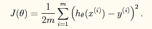
又线性回归的理论可以知道系统的损失函数如下所示：

其向量表达形式如下：

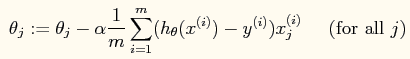
当使用梯度下降法进行参数的求解时，参数的更新公式如下：

实验结果：

测试学习率的结果如下：

由此可知，选用学习率为1时，可以到达很快的收敛速度，因此最终的程序中使用的学习率为1.

数据处理

Load the data for the training examples into your program and add the intercept term into your x matrix. Recall that the command in Matlab/Octave for adding a column of ones is

x = [ones(m, 1), x];

Take a look at the values of the inputs and note that the living areas are about 1000 times the number of bedrooms. This difference means that preprocessing the inputs will significantly increase gradient descent's efficiency.

In your program, scale both types of inputs by their standard deviations and set their means to zero. In Matlab/Octave, this can be executed with

sigma = std(x);
mu = mean(x);
x(:,2) = (x(:,2) - mu(2))./ sigma(2);
x(:,3) = (x(:,3) - mu(3))./ sigma(3);

实验代码

%% 方法一：梯度下降法
x = load('ex3x.dat');
y = load('ex3y.dat');

x = [ones(size(x,1),1) x];
meanx = mean(x);%求均值
sigmax = std(x);%求标准偏差
x(:,2) = (x(:,2)-meanx(2))./sigmax(2);
x(:,3) = (x(:,3)-meanx(3))./sigmax(3);

figure
itera_num = 100; %尝试的迭代次数
sample_num = size(x,1); %训练样本的次数
alpha = [0.01, 0.03, 0.1, 0.3, 1, 1.3];%因为差不多是选取每个3倍的学习率来测试，所以直接枚举出来
plotstyle = {'b', 'r', 'g', 'k', 'b--', 'r--'};

theta_grad_descent = zeros(size(x(1,:)));
for alpha_i = 1:length(alpha) %尝试看哪个学习速率最好
    theta = zeros(size(x,2),1); %theta的初始值赋值为0
    Jtheta = zeros(itera_num, 1);
    for i = 1:itera_num %计算出某个学习速率alpha下迭代itera_num次数后的参数       
        Jtheta(i) = (1/(2*sample_num)).*(x*theta-y)'*(x*theta-y);%Jtheta是个行向量
        grad = (1/sample_num).*x'*(x*theta-y);
        theta = theta - alpha(alpha_i).*grad;
    end
    plot(0:49, Jtheta(1:50),char(plotstyle(alpha_i)),'LineWidth', 2)%此处一定要通过char函数来转换
    hold on
    
    if(1 == alpha(alpha_i)) %通过实验发现alpha为1时效果最好，则此时的迭代后的theta值为所求的值
        theta_grad_descent = theta
    end
end
legend('0.01','0.03','0.1','0.3','1','1.3');
xlabel('Number of iterations')
ylabel('Cost function')

%下面是预测公式
price_grad_descend = theta_grad_descent'*[1 (1650-meanx(2))/sigmax(2) (3-meanx(3)/sigmax(3))]'
                                     
                                     
%%方法二：normal equations
x = load('ex3x.dat');
y = load('ex3y.dat');
x = [ones(size(x,1),1) x];

theta_norequ = inv((x'*x))*x'*y
price_norequ = theta_norequ'*[1 1650 3]'