In this chapter, we will cover:
- Filtering images using low-pass filters
- Filtering images using a median filter
- Applying directional filters to detect edges
- Computing the Laplacian of an image
图像各有不同因为他们有不一样的灰度级分布。如天空的灰度级不怎么变化,但是在一个对象非常多的图像里面,灰度级变化非常剧烈。因此,观察图像灰度级变化的频率组成了另一个处理图片的方式。Frequency domain(频域),观察图像灰度的分布,与空间域(Spatial domain)相对应。
Low frequency corresponds to areas where the image intensities vary slowly, while high frequencies are generated by rapid changes in intensities.
Note that since an image is a two-dimensional entity, it is made of both vertical frequencies (that is variations in the vertical directions) and horizontal frequencies (variations in the horizontal directions)。
A filter is an operation that amplifies certain bands of frequencies of an image while blocking (or reducing) other image frequency bands. A low-pass filter is therefore a filter which eliminates the highfrequency components of an image and reciprocally, a high-pass filter eliminates the low-pass components.
Filtering images using low-pass filters
The objective of such filters is to reduce the amplitude of the image variations.One simple way to achieve this goal is to replace each pixel by the average value of the pixels around. By doing this, the rapid intensity variations will be smoothed out and thus replaced by a more gradual transition.
The objective of the cv::blurfunction is to smooth an image by replacing each pixel by the average pixel value computed over a rectangular neighborhood. This low-pass filter is applied as follows:
cv::blur(image,result,cv::Size(5,5));
In some cases, it might be desirable to give more importance to the closer pixels in the neighborhood of a pixel. It is therefore possible to compute a weighted average in which nearby pixels are assigned a larger weight than ones further away. This can be achieved by using a weighted scheme that follows a Gaussian function (a "bell-shaped"function). The cv::GaussianBlur function applies such a filter and it is called as follows:
cv::GaussianBlur(image,result,cv::Size(5,5),1.5);
Use the following fuction to get the Gaussion Kernel:
cv::Mat gauss= cv::getGaussianKernel(9,sigma,CV_32F);
The function cv::sepFilter2D can be used to apply a general separable filter.
Consequently, to reduce the size of an image by half without adding annoying artifacts, you must first apply a low-pass filter to the original image and then throw away one column and row over two. This is exactly what the cv::pyrDownfunction does:
cv::Mat reducedImage; // to contain reduced image
cv::pyrDown(image,reducedImage); // reduce image size by half
This one uses a 5x5 Gaussian filter to low-pass the image. The reciprocal cv::pyrUp function that doubles the size of an image also exists.Of course, if you downsize an image and then upsize it, you will not recover the exact original image.
Note that there is also a more general cv:resizefunction that allows you to specify the size you want for the resulting image. You simply call it by specifying a new size that could be smaller or larger than the original image:
cv::Mat resizedImage; // to contain resized image
cv::resize(image,resizedImage,
cv::Size(image.cols/3,image.rows/3)); // 1/3 resizing
The function cv::boxFilterfilters an image with a square kernel made of 1s only. It is similar to the mean filter but without dividing the result by the number of coefficients.The cv::filter2D function lets you apply a linear filter to an image by inputting the kernel of your choice.
Filtering images using a median filter
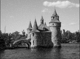
Since median filters are particularly useful to combat salt-and-pepper noise, we will use the image we created in the first recipe of Chapter 2and that is reproduced here:
The call to the median filtering function is done in a way similar to the other filters:
cv::medianBlur(image,result,5);
The resulting image is then as follows: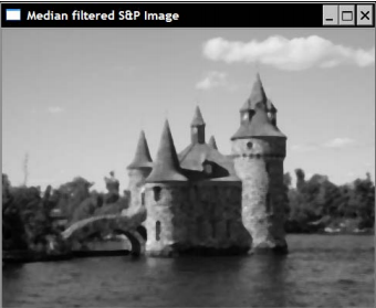
The median filter will simply compute the median value of this set, and the current pixel is then replaced by this median value. This explains why the filter is so efficient in eliminating of the salt-and-pepper noise. Indeed, when an outlier black or white pixel is present in a given pixel neighborhood, it is never selected as the median value (being rather maximal or minimal value) so it is always replaced by a neighboring value.
The median filter also has the advantage of preserving the sharpness of the edges. However, it washes out the textures in uniform regions (for example, the trees in the background).
Applying directional filters to detect edges
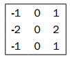
The filter we will use here is called the Sobel filter. It is said to be a directional filter because it only affects the vertical or the horizontal image frequencies depending on which kernel of the filter is used. OpenCV has a function that applies the Sobel operator on an image. The horizontal filter is called as follows:
cv::Sobel(image,sobelX,CV_8U,1,0,3,0.4,128);
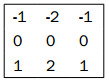
While vertical filtering is achieved by the following (and very similar) call:
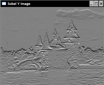
cv::Sobel(image,sobelY,CV_8U,0,1,3,0.4,128);
these have been chosen to produce an 8-bit image (CV_8U) representation of the output.The result of the horizontal Sobel operator is as follows:
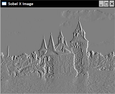
in this representation, a zero value corresponds to gray-level 128. Negative values are represented by darker pixels, while positive values are represented by brighter pixels. The vertical Sobel image is:
Since its kernel contains positive and negative values, the result of the Sobel filter is generally computed in a 16-bit signed integer image (CV_16S). The two results (vertical and horizontal) are then combined to obtain the norm of the Sobel filter:
// Compute norm of Sobel
cv::Sobel(image,sobelX,CV_16S,1,0);
cv::Sobel(image,sobelY,CV_16S,0,1);
cv::Mat sobel;
//compute the L1 norm
sobel= abs(sobelX)+abs(sobelY);
The Sobel norm can be conveniently displayed in an image using the optional rescaling parameter of the convertTo method in order to obtain an image in which zero values correspond to white, and higher values are assigned darker gray shades:
// Find Sobel max value
double sobmin, sobmax;
cv::minMaxLoc(sobel,&sobmin,&sobmax);
// Conversion to 8-bit image
// sobelImage = -alpha*sobel + 255
cv::Mat sobelImage;
sobel.convertTo(sobelImage,CV_8U,-255./sobmax,255);
The result can be seen in the following image:

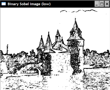
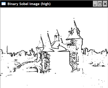
Looking at this image, it is now clear why this kind of operators are called edge detector. It is then possible to threshold this image in order to obtain a binary map showing the image contour. The following snippet creates the following image:
cv::threshold(sobelImage, sobelThresholded,
     threshold, 255, cv::THRESH_BINARY);
The Sobel operator is a classic edge detection linear filter that is based on a simple 3x3kernel which has the following structure:
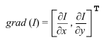
If we view the image as a two-dimensional function, the Sobel operator can then be seen as a measure of the variation of the image in the vertical and horizontal directions. In mathematical terms, this measure is called a gradientand it is defined as a 2D vector made of the function's first derivatives in two orthogonal directions:
The cv::Sobel function computes the result of the convolution of the image with a Sobel kernel. Its complete specification is as follows:
cv::Sobel(image, // input
     sobel, // output
     image_depth, // image type
     xorder,yorder, // kernel specification
     kernel_size, // size of the square kernel
     alpha, beta); // scale and offset
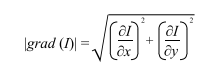
Since the gradient is a 2D vector, it has a norm and a direction. The norm of the gradient vector tells you what the amplitude of the variation is and it is normally computed as a Euclidean norm (also called L2 norm):
However, in image processing, we generally compute this norm as the sum of the absolute values. This is called the L1norm and it gives values close to the L2norm but at a much lower computational cost. This is what we did in this recipe, that is:
//compute the L1 norm
sobel= abs(sobelX)+abs(sobelY);
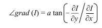
The gradient vector always points in the direction of the steepest variation. For an image, this means that the gradient direction will be orthogonal to the edge, pointing in the darker to brighter direction. Gradient angular direction is given by:
Most often, for edge detection, only the norm is computed. But if you require both the norm and the direction, then the following OpenCV function can be used:
// Sobel must be computed in floating points
cv::Sobel(image,sobelX,CV_32F,1,0);
cv::Sobel(image,sobelY,CV_32F,0,1);
// Compute the L2 norm and direction of the gradient
cv::Mat norm, dir;
cv::cartToPolar(sobelX,sobelY,norm,dir);
By default, the direction is computed in radians. Just add true as an additional argument in order to have them computed in degrees.
A binary edge map has been obtained by applying a threshold on the gradient magnitude. Choosing the right threshold is not an obvious task. If the threshold value is too low, too many (thick) edges will be retained, while if we select a more severe (higher) threshold, then broken edges will be obtained. As an illustration of this tradeoff situation, compare the preceding binary edge map with the following, o btained using a higher threshold value:
One possible alternative is to use the concept of hysteresis thresholding. This will be explained in the next chapter where we introduce the Canny operator.
- Computing the Laplacian of an image
The OpenCV function cv::Laplacian computes the Laplacian of an image. It is very similar to the cv::Sobel function. In fact, it uses the same basic function cv::getDerivKernels in order to obtain its kernel matrix. The only difference is that there is no derivative order parameters since these ones are by definition second order derivatives.
laplacianZC.h file as follows:
#if ! defined LAPLACIAN
#define  LAPLACIAN

#include <opencv2/core/core.hpp>
#include <opencv2/highgui/highgui.hpp>
#include <opencv2/imgproc/imgproc.hpp>

class LaplacianZC {
private:

                 // original image
                cv ::Mat img;
                 // 32-bit float image containing the Laplacian
                cv ::Mat laplace;
                 // Aperture size of the laplacian kernel
                 int aperture;

public:

                LaplacianZC () : aperture(3 ) {}

                 // Set the aperture size of the kernel
                 void setAperture( int a) {
                                aperture = a;
                 }

                 // Compute the floating point Laplacian
                cv ::Mat computeLaplacian( const cv:: Mat &image ) {

                                 // Compute Laplacian
                                cv ::Laplacian( image, laplace , CV_32F, aperture);

                                 // Keep local copy of the image
                                 // (used for zero-crossing)
                                img = image. clone();
                                 return laplace;
                 }

                 // Get the Laplacian result in 8-bit image
                 // zero corresponds to gray level 128
                 // if no scale is provided, then the max value will be
                 // scaled to intensity 255
                 // You must call computeLaplacian before calling this
                cv ::Mat getLaplacianImage( double scale = -1.0 ) {
                                 if ( scale < 0) {
                                                 double lapmin, lapmax;
                                                cv ::minMaxLoc( laplace, &lapmin, &lapmax );
                                                scale = 127 / std ::max(- lapmin, lapmax );
                                 }
                                cv ::Mat laplaceImage;
                                laplace .convertTo( laplaceImage, CV_8U , scale, 128);

                                 return laplaceImage;
                 }

};

#endif
main.cpp:
#include "laplacianZC.h"

int main() {

                cv ::Mat image = cv::imread ("../boldt.jpg", 0);
                 if (! image.data ) {
                                 return 0 ;
                 }

                cv ::namedWindow( "Original Image" );
                cv ::imshow( "Original Image" , image);

                 // Compute Laplacian using LaplacianZC class
                LaplacianZC laplacian ;
                laplacian .setAperture( 7);
                cv ::Mat flap = laplacian.computeLaplacian (image);
                cv ::Mat laplace = laplacian.getLaplacianImage ();

                cv ::namedWindow( "Laplacian Image" );
                cv ::imshow( "Laplacian Image" , laplace);

                cv ::waitKey( 0);

                 return 0 ;
}

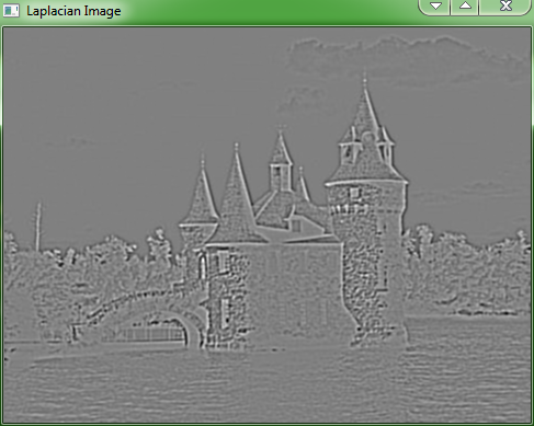
Formally, the Laplacianof a 2D function is defined as the sum of its second derivatives:

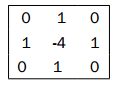
In its simplest form, it can be approximated by the following 3x3 kernel:
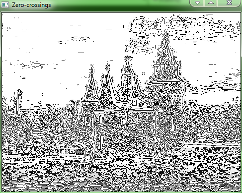
Consequently, a transition between a positive and a negative Laplacian value (or reciprocally) constitutes a good indicator of the presence of an edge.Another way to express this fact is to say that edges will be located at the zero-crossings of the Laplacian function.
A white box has been drawn in the following image to show the exact location of this region of interest:
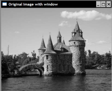
Now looking at the Laplacian values (7x7kernel) inside this window, we have:

If, as illustrated, you carefully follow the zero-crossings of the Laplacian (located between pixels of different signs), you obtain a curve which corresponds to the edge visible in the image window. This implies that, in principle, you can even detect the image edges at sub-pixel accuracy.
a simplified algorithm can be used to detect the approximate zero-crossing locations. This one proceeds as follows.Scan the Laplacian image and compare the current pixel with the one at its left. If the two pixels are of different signs, then declare a zero-crossing at the current pixel, if not, repeat the same test with the pixel immediately above. This algorithm is implemented by the following method which generates a binary image of zero-crossings:
// Get a binary image of the zero-crossing
                 // if the product of the two adjascent pixels is
                 // less than threshold then this zero-crsooing
                 // will be ignored
                cv ::Mat  getZeroCrossing( float threshold = 1.0) {

                                 // Create the iterators
                                cv ::Mat_< float>::const_iterator it = laplace. begin<float >() + laplace.step1 ();
                                cv ::Mat_< float>::const_iterator itend = laplace. end<float >();
                                cv ::Mat_< float>::const_iterator itup = laplace. begin<float >();

                                 // Binary image initialize to white
                                cv ::Mat binary( laplace.size (), CV_8U, cv::Scalar (255));
                                cv ::Mat_< uchar>::iterator itout = binary. begin<uchar >() + binary.step1 ();


                                 // negate the input threshold value
                                threshold *= - 1.0;

                                 for ( ; it != itend; ++it , ++ itup, ++itout) {

                                                 // if the product of two adjascent pixel is
                                                 // negative the there is a sign change
                                                 if (* it * *(it - 1) < threshold ) {
                                                                 *itout = 0; // horizontal zero-crossing
                                                 } else if (*it * *itup < threshold) {
                                                                 *itout = 0; // vertical zeor-crossing
                                                 }
                                 }
                                 return binary;
                 }
Using the function as follows:
double lapmin, lapmax;
                cv ::minMaxLoc( flap,&lapmin ,&lapmax);

                 // Compute and display the zero-crossing points
                cv ::Mat zeros;
                zeros = laplacian. getZeroCrossing(lapmax );
                cv ::namedWindow( "Zero-crossings" );
                cv ::imshow( "Zero-crossings" ,zeros);
Then we get the following result: