机器学习--线性单元回归--单变量梯度下降的实现
【线性回归】
如果要用一句话来解释线性回归是什么的话,那么我的理解是这样子的:
**线性回归,是从大量的数据中找出最优的线性(y=ax+b)拟合函数,通过数据确定函数中的未知参数,进而进行后续操作(预测)
**回归的概念是从统计学的角度得出的,用抽样数据去预估整体(回归中,是通过数据去确定参数),然后再从确定的函数去预测样本。
【损失函数】
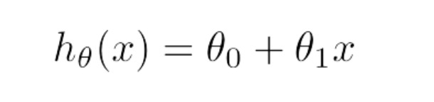
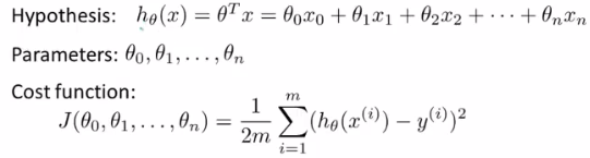
用线性函数去拟合数据,那么问题来了,到底什么样子的函数最能表现样本?对于这个问题,自然而然便引出了损失函数的概念,损失函数是一个用来评价样本数据与目标函数(此处为线性函数)拟合程度的一个指标。我们假设,线性函数模型为:
基于此函数模型,我们定义损失函数为:
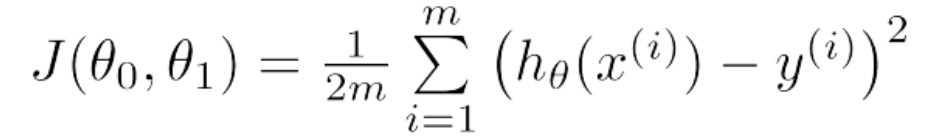
从上式中我们不难看出,损失函数是一个累加和(统计量)用来记录预测值与真实值之间的1/2方差,从方差的概念我们知道,方差越小说明拟合的越好。那么此问题进而演变称为求解损失函数最小值的问题,因为我们要通过样本来确定线性函数的中的参数θ_0和θ_1.
【梯度下降】
梯度下降算法是求解最小值的一种方法,但并不是唯一的方法。梯度下降法的核心思想就是对损失函数求偏导,从随机值(任一初始值)开始,沿着梯度下降的方向对θ_0和θ_1的迭代,最终确定θ_0和θ_1的值,注意,这里要同时迭代θ_0和θ_1(这一点在编程过程中很重要),具体迭代过程如下: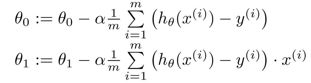
【Python代码实现】
那么下面我们使用python代码来实现线性回归的梯度下降。
#此处数据集,采用吴恩达第一次作业的数据集:ex1data1.txt
# -*- coding: utf-8 -*-
import numpy as np
import matplotlib.pyplot as plt
# 读取数据
def readData(path):
data = np.loadtxt(path, dtype=float, delimiter=',')
return data
# 损失函数,返回损失函数计算结果
def costFunction(theta_0, theta_1, x, y, m):
predictValue = theta_0 + theta_1 * x
return sum((predictValue - y) ** 2) / (2 * m)
# 梯度下降算法
# data:数据
# theta_0、theta_1:参数θ_0、θ_1
# iterations:迭代次数
# alpha:步长(学习率)
def gradientDescent(data, theta_0, theta_1, iterations, alpha):
eachIterationValue = np.zeros((iterations, 1))
x = data[:, 0]
y = data[:, 1]
m = data.shape[0]
for i in range(0, iterations):
hypothesis = theta_0 + theta_1 * x
temp_0 = theta_0 - alpha * ((1 / m) * sum(hypothesis - y))
temp_1 = theta_1 - alpha * (1 / m) * sum((hypothesis - y) * x)
theta_0 = temp_0
theta_1 = temp_1
costFunction_temp = costFunction(theta_0, theta_1, x, y, m)
eachIterationValue[i, 0] = costFunction_temp
return theta_0, theta_1, eachIterationValue
if __name__ == '__main__':
data = readData('ex1data1.txt')
iterations = 1500
plt.scatter(data[:, 0], data[:, 1], color='g', s=20)
# plt.show()
theta_0, theta_1, eachIterationValue = gradientDescent(data, 0, 0, iterations, 0.01)
hypothesis = theta_0 + theta_1 * data[:, 0]
plt.plot(data[:, 0], hypothesis)
plt.title("Fittingcurve")
plt.show()
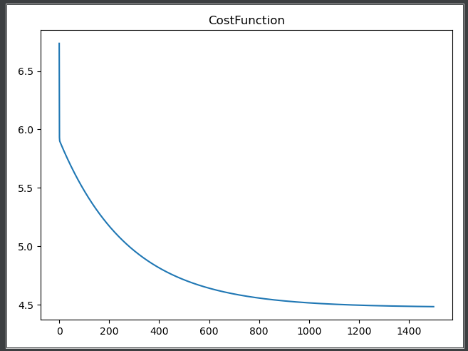
plt.plot(np.arange(iterations),eachIterationValue)
plt.title('CostFunction')
plt.show()
# 在这里我们使用向量的知识来写代码
# -*- coding: utf-8 -*-
import numpy as np
import matplotlib.pyplot as plt
"""
1.获取数据,并且将数据变为我们可以方便使用的数据格式
"""
def LoadFile(filename):
data = np.loadtxt(filename, delimiter=',', unpack=True, usecols=(0, 1))
X = np.transpose(np.array(data[:-1]))
y = np.transpose(np.array(data[-1:]))
X = np.insert(X, 0, 1, axis=1)
m = y.size
return X, y, m
"""
定义线性关系:Linear hypothesis function
"""
def h(theta, X):
return np.dot(X, theta)
"""
定义CostFunction
"""
def CostFunction(theta, X, y, m):
return float((1. / (2 * m)) * np.dot((h(theta, X) - y).T, (h(theta, X) - y)))
iterations = 1500
alpha = 0.01
def descendGradient(X, y, m, theta_start=np.array(2)):
theta = theta_start
CostVector = []
theta_history = []
for i in range(0, iterations):
tmptheta = theta
CostVector.append(CostFunction(theta, X, y, m))
theta_history.append(list(theta[:, 0]))
# 同步更新每一个theta的值
for j in range(len(tmptheta)):
tmptheta[j] = theta[j] - (alpha / m) * np.sum((h(theta, X) - y) * np.array(X[:, j]).reshape(m, 1))
theta = tmptheta
return theta, theta_history, CostVector
if __name__ == '__main__':
X, y, m = LoadFile('ex1data1.txt')
plt.figure(figsize=(10, 6))
plt.scatter(X[:, 1], y[:, 0], color='red')
theta = np.zeros((X.shape[1], 1))
theta, theta_history, CostVector = descendGradient(X, y, m, theta)
predictValue = h(theta, X)
plt.plot(X[:, 1], predictValue)
plt.xlabel('the value of x')
plt.ylabel('the value of y')
plt.title('the liner gradient descend')
plt.show()
plt.plot(range(len(CostVector)), CostVector, 'bo')
plt.grid(True)
plt.title("Convergence of Cost Function")
plt.xlabel("Iteration number")
plt.ylabel("Cost function")
plt.xlim([-0.05 * iterations, 1.05 * iterations])
plt.ylim([4, 7])
plt.title('CostFunction')
plt.show()
# 我们使用我们写好的线性模型去预测未知数据的情况,这样我们就可以得出一个属于我们自己的结果。
# 把我们线性模型预测的结果和实际的结果作一个对比,我们就可以看出实际结果是否真假性。
X, y, m = LoadFile('ex1data3.txt')
predictValue = h(theta, X)
print(predictValue)
# 这里我们可以得到我们的预测值,我们用建立好的模型去预测未知的模型情况。
‘’‘
[[1.16037866]
[3.98169165]]
’‘’
项目运行的结果为:
| 
 |
|
机器学习--多元线性回归--多变量梯度下降的实现
| 
|
| -------------------------------------------------------- |
| 
|
| 
|
梯度下降--特征缩放
通过特征缩放这个简单的方法,你将可以使得梯度下降的速度变得更快,收敛所迭代的次数变得更少。我们来看一下特征缩放的含义。
#Feature normalizing the columns (subtract mean, divide by standard deviation)
#Store the mean and std for later use
#Note don't modify the original X matrix, use a copy
stored_feature_means, stored_feature_stds = [], []
Xnorm = X.copy()
for icol in range(Xnorm.shape[1]):
    stored_feature_means.append(np.mean(Xnorm[:,icol]))
    stored_feature_stds.append(np.std(Xnorm[:,icol]))
    #Skip the first column
    if not icol: continue
    #Faster to not recompute the mean and std again, just used stored values
    Xnorm[:,icol] = (Xnorm[:,icol] - stored_feature_means[-1])/stored_feature_stds[-1]
学习率(alpha)
梯度下降的时候,我们有一个很重要的概念就是学习率的设定,在这里我们要明确一个概念,学习率可以反映梯度下降的情况。如果学习率太低,我们梯度下降的速率就会很慢。同时如果学习率太高,我们的梯度下降会错过最低点,theta的值不是最佳的,同时,可能不会收敛,一直梯度下去,值会越来越大。
那么我们应该选择一个多少大小的学习率是比较合适的呢?这里吴恩达老师给了一个建议,我们不妨参考。
......0.01、0.03、006、009、0.1、0.3、0.6......。综上所述,我们应该选择一个合适大小的学习率。
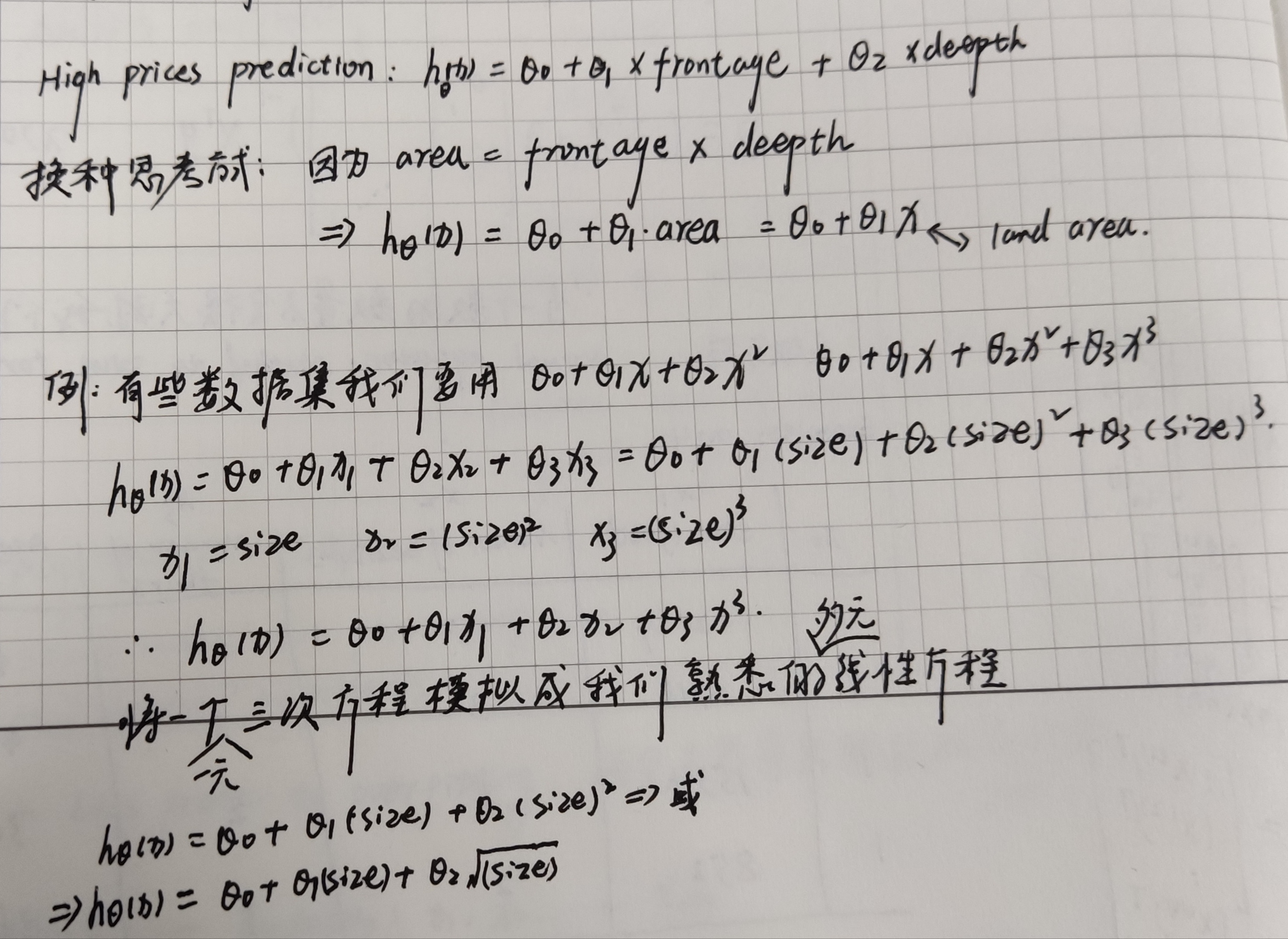
特征和多项式回归
| 
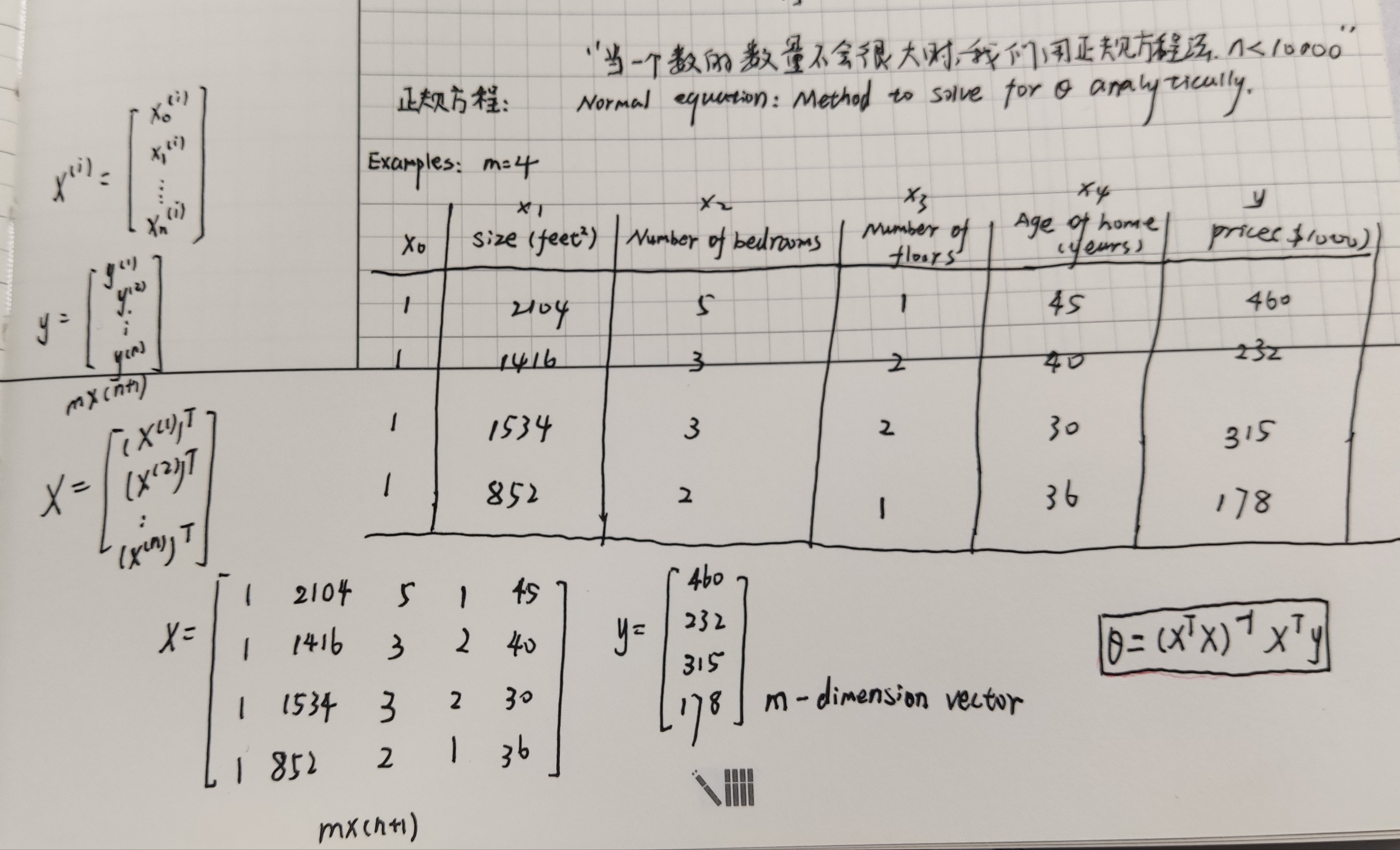
正规方程法(区别与迭代方法的直接求解)
| 
【Python代码实现多元的线性回归】
# -*- coding: utf-8 -*-
import numpy as np
import matplotlib.pyplot as plt

"""
1.获取数据的结果,使得数据是我们可以更好处理的数据
"""


def LoadFile(filename):
    data = np.loadtxt(filename, delimiter=',', usecols=(0, 1, 2), unpack=True)
    X = np.transpose(np.array(data[:-1]))
    y = np.transpose(np.array(data[-1:]))
    X = np.insert(X, 0, 1, axis=1)
    m = y.shape[0]
    return X, y, m


"""
2.构建线性函数
"""


def h(theta, X):
    return np.dot(X, theta)


"""
3.损失函数CostFunction
"""


def CostFunction(X, y, theta, m):
    return float((1. / (2 * m)) * np.dot((h(theta, X) - y).T, (h(theta, X) - y)))


"""
4.定义特征缩放的函数
因为数据集之间的差别比较的大,所以我们这里用可梯度下降--特征缩放
"""


def normal_feature(Xnorm):
    stored_feature_means, stored_feature_stds = [], []

    for icol in range(Xnorm.shape[1]):
        # 求平均值
        stored_feature_means.append(np.mean(Xnorm[:, icol]))
        # 求方差
        stored_feature_stds.append(np.std(Xnorm[:, icol]))
        # Skip the first column
        if not icol: continue
        # Faster to not recompute the mean and std again, just used stored values
        Xnorm[:, icol] = (Xnorm[:, icol] - stored_feature_means[-1]) / stored_feature_stds[-1]
    return Xnorm, stored_feature_means, stored_feature_stds


"""
5.定义梯度下降函数
"""
iterations = 1500
alpha = 0.01


def descendGradient(X, y, m, theta):
    CostVector = []
    theta_history = []
    for i in range(iterations):
        tmptheta = theta
        theta_history.append(list(theta[:, 0]))
        CostVector.append(CostFunction(X, y, theta, m))
        for j in range(len(tmptheta)):
            tmptheta[j, 0] = theta[j] - (alpha / m) * np.sum((h(theta, X) - y) * np.array(X[:, j]).reshape(m, 1))
        theta = tmptheta
    return theta, theta_history, CostVector


"""
6.定义绘图函数
"""


def plotConvergence(jvec):
    plt.figure(figsize=(10, 6))
    plt.plot(range(len(jvec)), jvec, 'bo')
    plt.grid(True)
    plt.title("Convergence of Cost Function")
    plt.xlabel("Iteration number")
    plt.ylabel("Cost function")
    plt.xlim([-0.05 * iterations, 1.05 * iterations])
    plt.ylim([4, 7])
    plt.show()


if __name__ == '__main__':
    X, y, m = LoadFile('ex1data2.txt')
    plt.figure(figsize=(10, 6))
    plt.grid(True)
    plt.xlim([-100, 5000])
    plt.hist(X[:, 0], label='col1')
    plt.hist(X[:, 1], label='col2')
    plt.hist(X[:, 2], label='col3')
    plt.title('Clearly we need feature normalization.')
    plt.xlabel('Column Value')
    plt.ylabel('Counts')
    plt.legend()
    plt.show()

    Xnorm = X.copy()
    Xnorm, stored_feature_means, stored_feature_stds = normal_feature(Xnorm)

    plt.grid(True)
    plt.xlim([-5, 5])
    plt.hist(Xnorm[:, 0], label='col1')
    plt.hist(Xnorm[:, 1], label='col2')
    plt.hist(Xnorm[:, 2], label='col3')
    plt.title('Feature Normalization Accomplished')
    plt.xlabel('Column Value')
    plt.ylabel('Counts')
    plt.legend()
    plt.show()

    theta = np.zeros((Xnorm.shape[1], 1))
    theta, theta_history, CostVector = descendGradient(Xnorm, y, m, theta)
    plotConvergence(CostVector)

    print("Check of result: What is price of house with 1650 square feet and 3 bedrooms?")
    ytest = np.array([1650., 3.])
    # To "undo" feature normalization, we "undo" 1650 and 3, then plug it into our hypothesis
    # 对于每次传来的一个数字我们读进行适当的特征缩放的功能
    ytestscaled = [(ytest[x] - stored_feature_means[x + 1]) / stored_feature_stds[x + 1] for x in range(len(ytest))]
    ytestscaled.insert(0, 1)
    print(ytestscaled)
    # 预测未知的值,通过我们已经建立好的模型来预测未知的值。
    print("$%0.2f" % float(h(theta, ytestscaled)))

    # 输出的结果为:
    [1, -0.4460438603276164, -0.2260933675776883]
	$293098.15
    输出的截图这里就不截图了
【python代码实现一元和多元线性回归汇总】
%matplotlib inline
import numpy as np
import matplotlib.pyplot as plt

cols = np.loadtxt(datafile,delimiter=',',usecols=(0,1),unpack=True) #Read in comma separated data

#Form the usual "X" matrix and "y" vector
X = np.transpose(np.array(cols[:-1]))

y = np.transpose(np.array(cols[-1:]))
m = y.size # number of training examples
#Insert the usual column of 1's into the "X" matrix
X = np.insert(X,0,1,axis=1)
print(X)

#Plot the data to see what it looks like
plt.figure(figsize=(10,6))
plt.plot(X[:,1],y[:,0],'rx',markersize=10)
plt.grid(True) #Always plot.grid true!
plt.ylabel('Profit in $10,000s')
plt.xlabel('Population of City in 10,000s')

iterations = 1500
alpha = 0.01

def h(theta,X): #Linear hypothesis function
    return np.dot(X,theta)

def computeCost(mytheta,X,y): #Cost function
    """
    theta_start is an n- dimensional vector of initial theta guess
    X is matrix with n- columns and m- rows
    y is a matrix with m- rows and 1 column
    """
    #note to self: *.shape is (rows, columns)
    return float((1./(2*m)) * np.dot((h(mytheta,X)-y).T,(h(mytheta,X)-y)))

#Test that running computeCost with 0's as theta returns 32.07:

initial_theta = np.zeros((X.shape[1],1)) #(theta is a vector with n rows and 1 columns (if X has n features) )
print(computeCost(initial_theta,X,y))


#Actual gradient descent minimizing routine
def descendGradient(X, theta_start = np.zeros(2)):
    """
    theta_start is an n- dimensional vector of initial theta guess
    X is matrix with n- columns and m- rows
    """
    theta = theta_start
    jvec = [] #Used to plot cost as function of iteration
    thetahistory = [] #Used to visualize the minimization path later on
    for meaninglessvariable in range(iterations):
        tmptheta = theta
        jvec.append(computeCost(theta,X,y))
        # Buggy line
        #thetahistory.append(list(tmptheta))
        # Fixed line
        thetahistory.append(list(theta[:,0]))
        #Simultaneously updating theta values
        for j in range(len(tmptheta)):
            tmptheta[j] = theta[j] - (alpha/m)*np.sum((h(initial_theta,X) - y)*np.array(X[:,j]).reshape(m,1))
        theta = tmptheta
    return theta, thetahistory, jvec

#Actually run gradient descent to get the best-fit theta values
initial_theta = np.zeros((X.shape[1],1))
theta, thetahistory, jvec = descendGradient(X,initial_theta)

#Plot the convergence of the cost function
def plotConvergence(jvec):
    plt.figure(figsize=(10,6))
    plt.plot(range(len(jvec)),jvec,'bo')
    plt.grid(True)
    plt.title("Convergence of Cost Function")
    plt.xlabel("Iteration number")
    plt.ylabel("Cost function")
    dummy = plt.xlim([-0.05*iterations,1.05*iterations])
    #dummy = plt.ylim([4,8])


plotConvergence(jvec)
dummy = plt.ylim([4,7])


#Plot the line on top of the data to ensure it looks correct
def myfit(xval):
    return theta[0] + theta[1]*xval
plt.figure(figsize=(10,6))
plt.plot(X[:,1],y[:,0],'rx',markersize=10,label='Training Data')
plt.plot(X[:,1],myfit(X[:,1]),'b-',label = 'Hypothesis: h(x) = %0.2f + %0.2fx'%(theta[0],theta[1]))
plt.grid(True) #Always plot.grid true!
plt.ylabel('Profit in $10,000s')
plt.xlabel('Population of City in 10,000s')
plt.legend()


#Import necessary matplotlib tools for 3d plots
from mpl_toolkits.mplot3d import axes3d, Axes3D
from matplotlib import cm
import itertools

fig = plt.figure(figsize=(12,12))
ax = fig.gca(projection='3d')

xvals = np.arange(-10,10,.5)
yvals = np.arange(-1,4,.1)
myxs, myys, myzs = [], [], []
for david in xvals:
    for kaleko in yvals:
        myxs.append(david)
        myys.append(kaleko)
        myzs.append(computeCost(np.array([[david], [kaleko]]),X,y))

scat = ax.scatter(myxs,myys,myzs,c=np.abs(myzs),cmap=plt.get_cmap('YlOrRd'))

plt.xlabel(r'$	heta_0$',fontsize=30)
plt.ylabel(r'$	heta_1$',fontsize=30)
plt.title('Cost (Minimization Path Shown in Blue)',fontsize=30)
plt.plot([x[0] for x in thetahistory],[x[1] for x in thetahistory],jvec,'bo-')
plt.show()


datafile = 'data/ex1data2.txt'
#Read into the data file
cols = np.loadtxt(datafile,delimiter=',',usecols=(0,1,2),unpack=True) #Read in comma separated data
#Form the usual "X" matrix and "y" vector
X = np.transpose(np.array(cols[:-1]))
y = np.transpose(np.array(cols[-1:]))
m = y.size # number of training examples
#Insert the usual column of 1's into the "X" matrix
X = np.insert(X,0,1,axis=1)

#Quick visualize data
plt.grid(True)
plt.xlim([-100,5000])
dummy = plt.hist(X[:,0],label = 'col1')
dummy = plt.hist(X[:,1],label = 'col2')
dummy = plt.hist(X[:,2],label = 'col3')
plt.title('Clearly we need feature normalization.')
plt.xlabel('Column Value')
plt.ylabel('Counts')
dummy = plt.legend()

#Feature normalizing the columns (subtract mean, divide by standard deviation)
#Store the mean and std for later use
#Note don't modify the original X matrix, use a copy
stored_feature_means, stored_feature_stds = [], []
Xnorm = X.copy()
for icol in range(Xnorm.shape[1]):
    stored_feature_means.append(np.mean(Xnorm[:,icol]))
    stored_feature_stds.append(np.std(Xnorm[:,icol]))
    #Skip the first column
    if not icol: continue
    #Faster to not recompute the mean and std again, just used stored values
    Xnorm[:,icol] = (Xnorm[:,icol] - stored_feature_means[-1])/stored_feature_stds[-1]

#Quick visualize the feature-normalized data
plt.grid(True)
plt.xlim([-5,5])
dummy = plt.hist(Xnorm[:,0],label = 'col1')
dummy = plt.hist(Xnorm[:,1],label = 'col2')
dummy = plt.hist(Xnorm[:,2],label = 'col3')
plt.title('Feature Normalization Accomplished')
plt.xlabel('Column Value')
plt.ylabel('Counts')
dummy = plt.legend()

#Run gradient descent with multiple variables, initial theta still set to zeros
#(Note! This doesn't work unless we feature normalize! "overflow encountered in multiply")
initial_theta = np.zeros((Xnorm.shape[1],1))
theta, thetahistory, jvec = descendGradient(Xnorm,initial_theta)

#Plot convergence of cost function:
plotConvergence(jvec)


#print "Final result theta parameters:
",theta
print ("Check of result: What is price of house with 1650 square feet and 3 bedrooms?")
ytest = np.array([1650.,3.])
#To "undo" feature normalization, we "undo" 1650 and 3, then plug it into our hypothesis
# 对于每次传来的一个数字我们读进行适当的特征缩放的功能
ytestscaled = [(ytest[x]-stored_feature_means[x+1])/stored_feature_stds[x+1] for x in range(len(ytest))]
ytestscaled.insert(0,1)
print ("$%0.2f" % float(h(theta,ytestscaled)))

from numpy.linalg import inv
#Implementation of normal equation to find analytic solution to linear regression
def normEqtn(X,y):
    #restheta = np.zeros((X.shape[1],1))
    return np.dot(np.dot(inv(np.dot(X.T,X)),X.T),y)

print ("Normal equation prediction for price of house with 1650 square feet and 3 bedrooms")
print ("$%0.2f" % float(h(normEqtn(X,y),[1,1650.,3])))