1、《BAM: Bottleneck Attention Module》
在这篇文章中,作者提出了新的Attention模型——瓶颈注意模块,通过分离的两个路径channel和spatial得到attention map,减少计算开销和参数开销。

针对输入特征F,通过两个通道,一个是通道Mc一个是空间Ms。
通道注意力分支:与SENet基本一致,每个通道都包含一个特定的特征响应,强调关注什么特征(what)
(1)先做全局平均池化,生成一个通道向量Fc∈RC×1×1,向量在每个通道中对全局信息进行编码。
(2)为了从通道向量Fc估计通道间的注意力,使用带有一个隐含 层的多层感知器(MLP),隐藏的激活大小设置为RC/r×1×1,其中r是衰减率。
(3)在MLP之后,添加一个批量归一化层( BN)来调整空间分支输出的尺度。
空间注意力分支:强调或抑制在不同空间位置的特征(where),利用膨胀卷积来高效地扩大感受野,空间注意力分支采用了ResNet提出的“瓶颈结构”
(1)首先,使用1×1卷积将特征F降维得到RC/r×H×W。
(2)然后,使用与通道分支相同的衰减率r,衰减后,应用两个3×3膨胀卷积来有效地利用上下文信息。
(3)最后,利用1×1卷积将特征再次简化为R1×H×W空间注意力图。
(4)为了调整尺度,在空间分支的末端应用BN批量标准化层。
最后将两个分支的注意力相加(用到广播机制)后进行sigmoid函数获得最后的注意力映射M(F),M(F)与F进行点乘后再与F相加,应用残差学校和注意力机制。
  1 import torch
  2 from torch import nn
  3 from torch.nn import init
  4
  5
  6 # 通道注意力+空间注意力的改进版
  7 # 方法出处 2018 BMCV 《BAM: Bottleneck Attention Module》
  8 # 展平层
  9 class Flatten(nn.Module):
 10     def __init__(self):
 11         super(Flatten, self).__init__()
 12
 13     # 将输入的x,假如它是[B,C,H,W]维度的特征图
 14     # 其中B代表批大小
 15     # C代表通道数
 16     # H,W代表高和宽
 17     # 展平层将特征图展平为[B,C*H*W]
 18     # 其中每一个是一个行向量
 19     # 方便输入到下一个全连接层中
 20     def forward(self, x):
 21         return x.view(x.shape[0], -1)
 22
 23
 24 # 通道注意力
 25 class ChannelAttention(nn.Module):
 26     # 网络层的初始化
 27     def __init__(self, channel, reduction=16, num_layers=3):
 28         super(ChannelAttention, self).__init__()
 29         # 自适应平均池化
 30         # 将特征图的维度,假设是[B,C,H,W]
 31         # 平均池化到[B,C,1,1]
 32         # 相当于将切片矩阵H,W
 33         # 先按行相加
 34         # 在按列相加
 35         self.avgpool = nn.AdaptiveAvgPool2d(1)
 36         # 通道注意力中的多个全连接层的通道参数
 37         # gate_channels是个列表
 38         # 其中存放如下的数字
 39         # [channel,channel//reduction,channel//reduction,...(这里由num_layers控制,就是你想有多少个中间层)
 40         # channel]最后没有改变输入的通道数
 41         # 因为最后要按照通道数乘以通道权重
 42         gate_channels = [channel]
 43         gate_channels += [channel // reduction] * num_layers
 44         gate_channels += [channel]
 45
 46         # 搭建全连接层计算通道注意力
 47         # Sequential以序列化的形式存储网络层
 48         self.ca = nn.Sequential()
 49         # 首先加入一个展平层,方便输入到后面的全连接层中
 50         self.ca.add_module('flatten', Flatten())
 51         # 循环依次就加入一个全连接层组合
 52         # 这个全连接组合包括
 53         # nn.Linear(channel,channel//reduction)或者
 54         # nn.Linear(channel//reduction,channel//reduction)形式的隐藏层
 55         # 紧接着全连接层之后的正则化层nn.BatchNorm1d因为输出的是向量所以用1d的正则化层
 56         # 然后是激活层
 57         for i in range(len(gate_channels) - 2):
 58             self.ca.add_module('fc%d' % i, nn.Linear(gate_channels[i], gate_channels[i + 1]))
 59             self.ca.add_module('bn%d' % i, nn.BatchNorm1d(gate_channels[i + 1]))
 60             self.ca.add_module('relu%d' % i, nn.ReLU())
 61         # 最后将通道数还原的全连接层
 62         self.ca.add_module('last_fc', nn.Linear(gate_channels[-2], gate_channels[-1]))
 63
 64     # 前向传递建立计算图
 65     def forward(self, x):
 66         # 首先进行池化
 67         res = self.avgpool(x)
 68         # 然后通过全连接层
 69         # 计算出不同通道之间的相似性信息
 70         res = self.ca(res)
 71         # 改变通道注意力结果到与输入的特征图统一维度
 72         # 方便后面的相乘运算
 73         res = res.unsqueeze(-1).unsqueeze(-1).expand_as(x)
 74         return res
 75
 76
 77 # 空间注意力
 78 class SpatialAttention(nn.Module):
 79     def __init__(self, channel, reduction=16, num_layers=3, dia_val=2):
 80         super(SpatialAttention, self).__init__()
 81         # 空间注意力中中间的卷积层
 82         self.sa = nn.Sequential()
 83         # 首先是1*1的卷积层
 84         # 1*1的卷积层不改变卷积层的输入的宽高
 85         # 只是改变输入的通道数
 86         self.sa.add_module('conv_reduce1',
 87                            nn.Conv2d(kernel_size=1, in_channels=channel, out_channels=channel // reduction))
 88         self.sa.add_module('bn_reduce1', nn.BatchNorm2d(channel // reduction))
 89         self.sa.add_module('relu_reduce1', nn.ReLU())
 90         # 然后是3个3*3的卷积层
 91         # 这里指定了使用空洞卷积
 92         # 普通的卷积,卷积核之间的元素之间是相邻的
 93         # 在空洞卷积中,卷积核之间的元素会间隔指定的距离
 94         # 这个距离由我们自己指定
 95         # 因为元素之间存在空隙
 96         # 所以叫做空洞卷积
 97         # 普通卷积输出宽高的计算公式
 98         # 输出的高=(输入的高+2*padding-卷积核大小)/卷积步幅+1
 99         # 带入参数可知这些3*3的卷积核也没有改变输入的宽高
100         # 但是这里的卷积层指定了空洞卷积
101         # 计算公式为
102         # 输出的高=(输入的高+2*padding-空洞距离(卷积核大小-1)-1)/卷积步幅+1
103         # 带入参数
104         # 输出的高=输入的高-2
105         # 3次之后宽,高就变成1*1
106         for i in range(num_layers):
107             self.sa.add_module('conv_%d' % i, nn.Conv2d(kernel_size=3, in_channels=channel // reduction,
108                                                         out_channels=channel // reduction, padding=1, dilation=dia_val))
109             self.sa.add_module('bn_%d' % i, nn.BatchNorm2d(channel // reduction))
110             self.sa.add_module('relu_%d' % i, nn.ReLU())
111         # 最后是1*1的卷积层
112         # 输出通道是1
113         # 最后空间注意力维度是[B,1,1,1]
114         self.sa.add_module('last_conv', nn.Conv2d(channel // reduction, 1, kernel_size=1))‘’
115     #前向传递,建立计算图
116     def forward(self, x):
117         #计算空间注意力
118         res = self.sa(x)
119         #同理要转换成和输入相同的维度
120         #方便和通道注意力的结果相加
121         res = res.expand_as(x)
122         return res
123
124
125 # BAM整体模型
126 class BAMBlock(nn.Module):
127     #初始化层
128     def __init__(self, channel=512, reduction=16, dia_val=2):
129         super().__init__()
130         #计算通道注意力
131         self.ca = ChannelAttention(channel=channel, reduction=reduction)
132         #计算空间注意力
133         self.sa = SpatialAttention(channel=channel, reduction=reduction, dia_val=dia_val)
134         #激活层
135         self.sigmoid = nn.Sigmoid()
136     #初始化网络层权重
137     def init_weights(self):
138         for m in self.modules():
139             if isinstance(m, nn.Conv2d):
140                 init.kaiming_normal_(m.weight, mode='fan_out')
141                 if m.bias is not None:
142                     init.constant_(m.bias, 0)
143             elif isinstance(m, nn.BatchNorm2d):
144                 init.constant_(m.weight, 1)
145                 init.constant_(m.bias, 0)
146             elif isinstance(m, nn.Linear):
147                 init.normal_(m.weight, std=0.001)
148                 if m.bias is not None:
149                     init.constant_(m.bias, 0)
150     #前向传递
151     def forward(self, x):
152         b, c, _, _ = x.size()
153         #通道注意力结果
154         sa_out = self.sa(x)
155         #空间注意力结果
156         ca_out = self.ca(x)
157         #激活
158         weight = self.sigmoid(sa_out + ca_out)
159         #这里有个残差连接x+weight*x
160         out = (1 + weight) * x
161         return out
162
163
164 if __name__ == '__main__':
165     # 可以将input看作一个特征图
166     input = torch.randn(50, 512, 7, 7)
167     # 捕获不同特征图不同通道之间的关系
168     bam = BAMBlock(channel=512, reduction=16, dia_val=2)
169     output = bam(input)
170     print(output.shape)
2、《Dual Attention Network for Scene Segmentation》
论文:https://openaccess.thecvf.com/content_CVPR_2019/papers/Fu_Dual_Attention_Network_for_Scene_Segmentation_CVPR_2019_paper.pdf
代码:https://github.com/junfu1115/DANet/
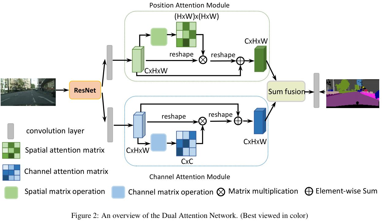
这个模型是对ResNet的改进,预处理时去除了原模型的下采样后应用扩展卷机得到特征图,变为原始图的1/8;再将该特征图分别输入到Position Attention模块与Channel Attention模块中分别获取到像素间的全局特征和通道间的全局特征,最后将两个全局特征进行融合得到最终的特征表示,再通过一个卷积层得到最终的语义分割结果图。
位置注意力模块:

文中运用了自注意力机制,BCD表示的是特征图A,都采用reshape操作变为二维矩阵C*N,N是H*W,三个矩阵对应于自注意力机制的Q,K,V。
(1)计算像素间的相似性矩阵,QT*K得到大小为N*N的相似性矩阵;
(2)对相似性矩阵使用softmax函数,得到每个影响该像素的相对因子;
(3)将得到的相似性矩阵与V矩阵相乘,最终得到C*N的特征表示;
(4)将最终得到的新的特征矩阵进行reshape操作,得到大小为C*H*W的重新编码的特征图,再与原始特征图相加得到最终的位置注意力的输出。
通道注意力模块:

同样,将A分成三块,分别表示注意力机制K,V,Q。
(1)计算像素间的相似性矩阵,其过程就是通过QT*K,也就是(C*N)矩阵乘上(N*C)矩阵得到了大小为N*N的像素间相似性矩阵。
(2)对相似性矩阵进行softmax操作,得到权重;
(3)将权重与V矩阵相乘,得到C*N的特征表示;
(4)将特征表示进行reshape操作,得到大小为C*H*W的特征图,将特征图与原始图进行相加得到最终通道注意力模块的输出。
最终将两个注意力机制提取的特征图元素级相加输入到一个卷积层得到最终的图像分割结果。
3、《ECA-Net: Efficient Channel Attention for Deep Convolutional Neural Networks》
论文:https://arxiv.org/abs/1910.03151
代码:https://github.com/BangguWu/ECANet
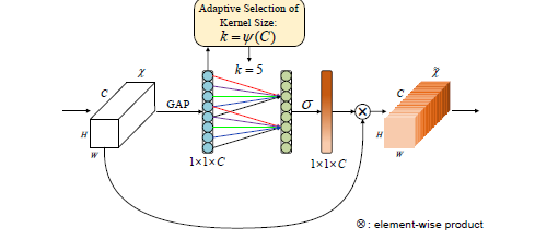
ECA是SENet的扩展,认为两个FC层的维度缩减不利于通道注意力的权重学习。SE是全局的注意力,ECA是局部的注意力。
ECA-Net的结构如下图所示:(1)global avg pooling产生1 ∗ 1 ∗ C 大小的feature maps;(2)计算得到自适应的kernel_size;(3)应用kernel_size于一维卷积中,得到每个channel的weight。
 1 import torch
 2 from torch import nn
 3 from torch.nn.parameter import Parameter
 4
 5 class eca_layer(nn.Module):
 6     """Constructs a ECA module.
 7     Args:
 8         channel: Number of channels of the input feature map
 9         k_size: Adaptive selection of kernel size
10     """
11     def __init__(self, channel, k_size=3):
12         super(eca_layer, self).__init__()
13         self.avg_pool = nn.AdaptiveAvgPool2d(1)
14         self.conv = nn.Conv1d(1, 1, kernel_size=k_size, padding=(k_size - 1) // 2, bias=False)
15         self.sigmoid = nn.Sigmoid()
16
17     def forward(self, x):
18         # x: input features with shape [b, c, h, w]
19         b, c, h, w = x.size()
20
21         # feature descriptor on the global spatial information
22         y = self.avg_pool(x)
23
24         # Two different branches of ECA module
25         y = self.conv(y.squeeze(-1).transpose(-1, -2)).transpose(-1, -2).unsqueeze(-1)
26
27         # Multi-scale information fusion
28         y = self.sigmoid(y)
29
30         return x * y.expand_as(x)
4、《Improving Convolutional Networks with Self-Calibrated Convolutions》
论文:http://mftp.mmcheng.net/Papers/20cvprSCNet.pdf
代码:https://github.com/MCG-NKU/SCNet
本文提出了一种新颖的自校正卷积,该卷积它可以通过特征的内在通信达到扩增卷积感受野的目的,进而增强输出特征的多样性。
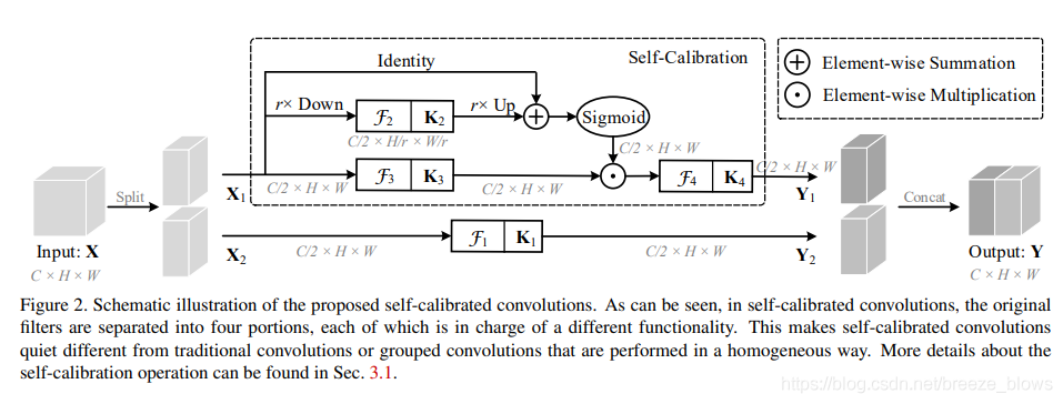
SCNet提出了一个自校准卷积,在通道上做注意力。论文提出在两个不同的尺度空间中进行卷积特征转换:原始尺度空间中的特征图(输入共享相同的分辨率)和下采样后的较小的潜在空间(自校准)。利用下采样后特征具有较大的视场,因此在较小的潜在空间中进行变换后的嵌入将用作参考,以指导原始特征空间中的特征变换过程。
整体框架如图所示,输入X先通过两个conv分成feature X1,X2。将卷积核分为四个部分,K1,K2,K3,K4,再通过以下自校准尺度空间:

上半部分:对特征X1使用平均池化下采样r倍,经过K2卷积核处理再进行双线性插值的上采样,将采样后的结果与X1进行相加后应用sigmoid函数,X1经过K3卷积后与sigmoid处理后的特征图点乘,这一步是校准,用学到的特征去校正卷积;最后经过K4卷积得到输出的特征Y1。
下半部分:对特征X2经过K1卷积提取得到特征Y2。
最后对两个尺度空间输出特征Y1,Y2进行拼接操作,得到最终输出特征Y。
  1 import torch
  2 import torch.nn as nn
  3 import torch.nn.functional as F
  4 import torch.utils.model_zoo as model_zoo
  5
  6 __all__ = ['SCNet', 'scnet50', 'scnet101']
  7
  8 model_urls = {
  9     'scnet50': 'https://backseason.oss-cn-beijing.aliyuncs.com/scnet/scnet50-dc6a7e87.pth',
 10     'scnet101': 'https://backseason.oss-cn-beijing.aliyuncs.com/scnet/scnet101-44c5b751.pth',
 11 }
 12
 13
 14 def conv3x3(in_planes, out_planes, stride=1, groups=1):
 15     """3x3 convolution with padding"""
 16     return nn.Conv2d(in_planes, out_planes, kernel_size=3, stride=stride,
 17                      padding=1, groups=groups, bias=False)
 18
 19
 20 def conv1x1(in_planes, out_planes, stride=1):
 21     """1x1 convolution"""
 22     return nn.Conv2d(in_planes, out_planes, kernel_size=1, stride=stride, bias=False)
 23
 24
 25 class SCConv(nn.Module):
 26     def __init__(self, planes, stride, pooling_r):
 27         super(SCConv, self).__init__()
 28         self.k2 = nn.Sequential(
 29             nn.AvgPool2d(kernel_size=pooling_r, stride=pooling_r),
 30             conv3x3(planes, planes),
 31             nn.BatchNorm2d(planes),
 32         )
 33         self.k3 = nn.Sequential(
 34             conv3x3(planes, planes),
 35             nn.BatchNorm2d(planes),
 36         )
 37         self.k4 = nn.Sequential(
 38             conv3x3(planes, planes, stride),
 39             nn.BatchNorm2d(planes),
 40             nn.ReLU(inplace=True),
 41         )
 42
 43     def forward(self, x):
 44         identity = x
 45
 46         out = torch.sigmoid(
 47             torch.add(identity, F.interpolate(self.k2(x), identity.size()[2:])))  # sigmoid(identity + k2)
 48         out = torch.mul(self.k3(x), out)  # k3 * sigmoid(identity + k2)
 49         out = self.k4(out)  # k4
 50
 51         return out
 52
 53
 54 class SCBottleneck(nn.Module):
 55     expansion = 4
 56     pooling_r = 4  # down-sampling rate of the avg pooling layer in the K3 path of SC-Conv.
 57
 58     def __init__(self, inplanes, planes, stride=1, downsample=None):
 59         super(SCBottleneck, self).__init__()
 60         planes = int(planes / 2)
 61
 62         self.conv1_a = conv1x1(inplanes, planes)
 63         self.bn1_a = nn.BatchNorm2d(planes)
 64
 65         self.k1 = nn.Sequential(
 66             conv3x3(planes, planes, stride),
 67             nn.BatchNorm2d(planes),
 68             nn.ReLU(inplace=True),
 69         )
 70
 71         self.conv1_b = conv1x1(inplanes, planes)
 72         self.bn1_b = nn.BatchNorm2d(planes)
 73
 74         self.scconv = SCConv(planes, stride, self.pooling_r)
 75
 76         self.conv3 = conv1x1(planes * 2, planes * 2 * self.expansion)
 77         self.bn3 = nn.BatchNorm2d(planes * 2 * self.expansion)
 78         self.relu = nn.ReLU(inplace=True)
 79         self.downsample = downsample
 80         self.stride = stride
 81
 82     def forward(self, x):
 83         residual = x
 84
 85         out_a = self.conv1_a(x)
 86         out_a = self.bn1_a(out_a)
 87         out_a = self.relu(out_a)
 88
 89         out_a = self.k1(out_a)
 90
 91         out_b = self.conv1_b(x)
 92         out_b = self.bn1_b(out_b)
 93         out_b = self.relu(out_b)
 94
 95         out_b = self.scconv(out_b)
 96
 97         out = self.conv3(torch.cat([out_a, out_b], dim=1))
 98         out = self.bn3(out)
 99
100         if self.downsample is not None:
101             residual = self.downsample(x)
102
103         out += residual
104         out = self.relu(out)
105
106         return out
107
108
109 class SCNet(nn.Module):
110     def __init__(self, block, layers, num_classes=1000):
111         super(SCNet, self).__init__()
112         self.inplanes = 64
113         self.conv1 = nn.Conv2d(3, 64, kernel_size=7, stride=2, padding=3,
114                                bias=False)
115         self.bn1 = nn.BatchNorm2d(self.inplanes)
116         self.relu = nn.ReLU(inplace=True)
117         self.maxpool = nn.MaxPool2d(kernel_size=3, stride=2, padding=1)
118         self.layer1 = self._make_layer(block, 64, layers[0])
119         self.layer2 = self._make_layer(block, 128, layers[1], stride=2)
120         self.layer3 = self._make_layer(block, 256, layers[2], stride=2)
121         self.layer4 = self._make_layer(block, 512, layers[3], stride=2)
122         self.avgpool = nn.AdaptiveAvgPool2d((1, 1))
123         self.fc = nn.Linear(512 * block.expansion, num_classes)
124
125         for m in self.modules():
126             if isinstance(m, nn.Conv2d):
127                 nn.init.kaiming_normal_(m.weight, mode='fan_out', nonlinearity='relu')
128             elif isinstance(m, nn.BatchNorm2d):
129                 nn.init.constant_(m.weight, 1)
130                 nn.init.constant_(m.bias, 0)
131
132     def _make_layer(self, block, planes, blocks, stride=1):
133         downsample = None
134         if stride != 1 or self.inplanes != planes * block.expansion:
135             downsample = nn.Sequential(
136                 conv1x1(self.inplanes, planes * block.expansion, stride),
137                 nn.BatchNorm2d(planes * block.expansion),
138             )
139
140         layers = []
141         layers.append(block(self.inplanes, planes, stride, downsample))
142         self.inplanes = planes * block.expansion
143         for _ in range(1, blocks):
144             layers.append(block(self.inplanes, planes))
145
146         return nn.Sequential(*layers)
147
148     def forward(self, x):
149         x = self.conv1(x)
150         x = self.bn1(x)
151         x = self.relu(x)
152         x = self.maxpool(x)
153
154         x = self.layer1(x)
155         x = self.layer2(x)
156         x = self.layer3(x)
157         x = self.layer4(x)
158
159         x = self.avgpool(x)
160         x = x.view(x.size(0), -1)
161         x = self.fc(x)
162
163         return x
164
165
166 def scnet50(pretrained=False, **kwargs):
167     """Constructs a SCNet-50 model.
168     Args:
169         pretrained (bool): If True, returns a model pre-trained on ImageNet
170     """
171     model = SCNet(SCBottleneck, [3, 4, 6, 3], **kwargs)
172     if pretrained:
173         model.load_state_dict(model_zoo.load_url(model_urls['scnet50']))
174     return model
175
176
177 def scnet101(pretrained=False, **kwargs):
178     """Constructs a SCNet-101 model.
179     Args:
180         pretrained (bool): If True, returns a model pre-trained on ImageNet
181     """
182     model = SCNet(SCBottleneck, [3, 4, 23, 3], **kwargs)
183     if pretrained:
184         model.load_state_dict(model_zoo.load_url(model_urls['scnet101']))
185     return model
186
187
188 if __name__ == '__main__':
189     images = torch.rand(1, 3, 224, 224)
190     model = scnet50(pretrained=False)
191     # model = model.cuda(0)
192     out = model(images)
193     print(model(images).size())
5、《Pyramid Split Attention》
链接:https://arxiv.org/abs/2105.14447
代码地址:https://github.com/murufeng/EPSANetAbstract & Introduction
PSA在SENet的基础上提出了多尺度特征图提取策略,整体架构如下所示:
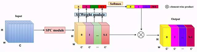
- Split and Concat (SPC)模块对通道进行切分,用于获得空间级多尺度特征图;
- SEWeight(SENet中的模块)被用于获得空间级视觉注意力向量,提取不同尺度特征图的通道注意力,得到每个不同尺度上的通道注意力向量;
- 使用Softmax函数用于再分配特征图权重向量,对多尺度通道注意力向量进行特征重新标定,得到新的多尺度通道交互之后的注意力权重;
- 元素相乘操作用于权重向量与原始特征图来获得最终结果响应图。
SPC模块:

如上图所示,首先将特征图切为X1,X2,X3,X4,k0、k1、k2和k3是不同卷积核参数,G0、G1、G2和G3是分组卷积的参数。特征图用多尺度分组卷积的方式提取不同尺度的特征图空间信息。整体可看做是模型采用不同卷积核提取多尺度目标特征,并采取Concat操作结合不同感受野下的多尺度特征。
6、《ResT: An Efficient Transformer for Visual Recognition》
(1)构建了一个memory-Efficient Multi-Head Self-Attention,它通过简单的depth-wise卷积,并在保持多头的多样性能力的同时,将交互投射到注意力头维度;
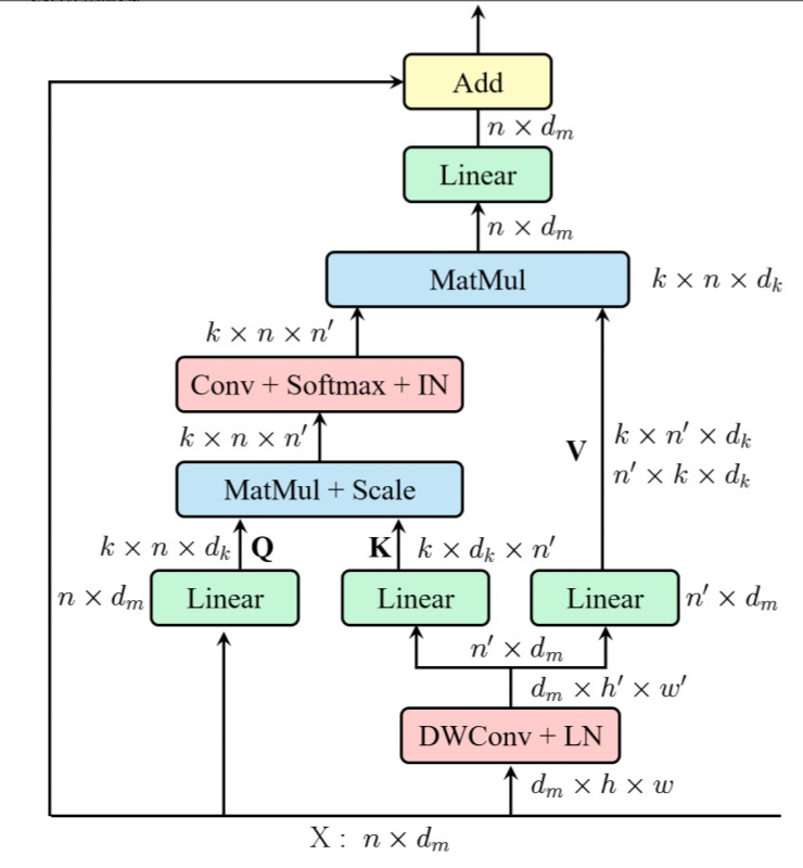
(2) 位置编码被构建为空间注意力,更灵活,可以处理任意大小的输入图像,无需插值或微调;
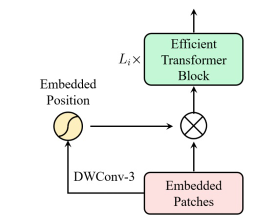
(3)不再在每个阶段开始时直接进行标记化,我们将patch嵌入设计为重叠的卷积运算堆栈,并在2D整形的标记图上大步前进。

7、《Beyond Self-attention: External Attention using Two Linear Layers for Visual Tasks》
本文作者提出了一个external attention模块,只需使用两个级联的线性层和两个归一化层即可轻松实现。我们首先通过计算query向量和外部可学习key存储器之间的点积来计算注意力图,然后通过将此注意力图与另一个外部可学习value存储器相乘来生成新的特征图。

图中(a)和(b)分别表示经典的self-attention和简化版self-attention。
自注意力机制是一个N−to−N的注意力矩阵,可视化像素之间的关系,可以发现这种相关性是比较稀疏的,即很多是冗余信息。因此清华团队提出了一个外部注意力模块。
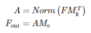
它的注意力计算是在输入像素与一个外部记忆单元M∈RS×d之间:

注意与自注意力机制不同,A是从先验信息得来的注意力特征图,Norm操作和自注意力一样。最终,通过A来更新M。
另外,我们用两种不同的记忆单元:Mk和Mv来增加网络的建模能力。
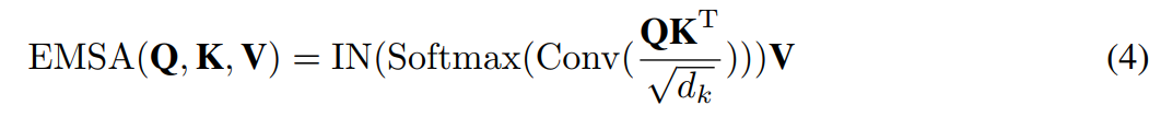
最终外部注意力机制的计算公式为:
经过上面的公式,外部注意力机制的复杂度大大降低。