把之前学习xgb过程中查找的资料整理分享出来,方便有需要的朋友查看,求大家点赞支持,哈哈哈
作者:tangg, qq:577305810
一、Boosting算法
boosting算法有许多种具体算法,包括但不限于ada boosting GBDT XGBoost .
所谓 Boosting ,就是将弱分离器 f_i(x) 组合起来形成强分类器 F(x) 的一种方法。
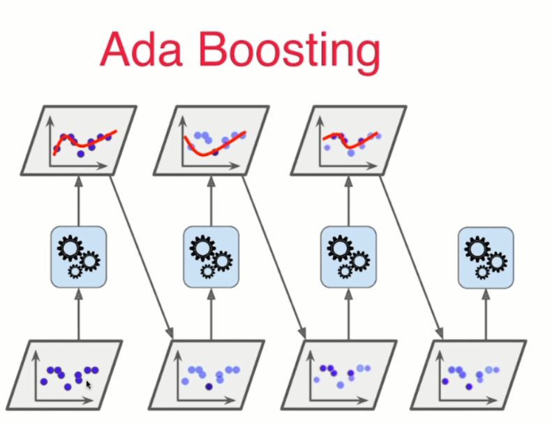
1. Ada boosting
每个子模型模型都在尝试增强(boost)整体的效果,通过不断的模型迭代,更新样本点的权重
Ada Boosting没有oob(out of bag ) 的样本,因此需要进行 train_test_split
原始数据集 》 某种算法拟合,会 产生错误 》 根据上个模型预测结果,更新样本点权重(预测错误的结果权重增大) 》 再次使用模型进行预测 》重复上述过程,继续重点训练错误的预测样本点
每一次生成的子模型,都是在生成拟合结果更好的模型,
(用的数据点都是相同的,但是样本点具有不同的权重值)
需要指定 Base Estimator
from sklearn.ensemble import AdaBoostClassifier
from sklearn.tree import DecisionTreeClassifier

ada_clf = AdaBoostClassifier(DecisionTreeClassifier(max_depth=2), n_estimators=500)
ada_clf.fit(X_train, y_train)

ada_clf.score(X_test, y_test)
2. Gradient Boosting(GBDT)
Gradient Boosting 又称为 DBDT (gradient boosting decision tree )
训练一个模型m1, 产生错误e1
针对e1训练第二个模型m2, 产生错误e2
针对e2训练第二个模型m3, 产生错误e3
......
最终的预测模型是:(m1+m2+m3+...)
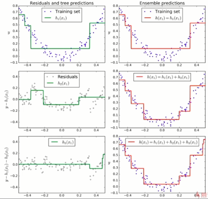
Gradient Boosting是基于决策树的,不用指定Base Estimator
from sklearn.ensemble import GradientBoostingClassifier

gb_clf = GradientBoostingClassifier(max_depth=2, n_estimators=30)
gb_clf.fit(X_train, y_train)
gb_clf.score(X_test, y_test)
3.XGBoost
这个算法的Base Estimator是基于decision tree的
Xgboost是在GBDT的基础上进行改进,使之更强大,适用于更大范围
xgboost可以用来确定特征的重要程度
强烈推荐博客园上【战争热诚】写的一篇介绍xgboost算法的文章,
非常详细地介绍了xgboost的优点、安装、xgboost参数的含义、使用xgboost实例代码、保存训练好的模型、并介绍了xgboost参数调优的一般流程。
然而,,,我发现该作者好像也是转载的,怪不得有些地方看不懂,还缺少代码。不过是中文的有助于理解。
文章原文链接如下:
Complete Guide to Parameter Tuning in XGBoost with codes in Python
文中提到的数据的github仓库地址:
Parameter_Tuning_GBM_with_Example
另外一篇,掘金上不错的文章:
3.1 xgboost模型参数
模型参数总体上分为3类:(this part is talked about 原生接口 params )
1. 通用参数
- booster[default=gbtree]
- 有两种模型可以选择gbtree和gblinear。gbtree使用基于树的模型进行提升计算,gblinear使用线性模型进行提升计算。
缺省值为gbtree
- 有两种模型可以选择gbtree和gblinear。gbtree使用基于树的模型进行提升计算,gblinear使用线性模型进行提升计算。
- silent [default=0]
- 取0时表示打印出运行时信息,取1时表示以缄默方式运行,不打印运行时的信息。
缺省值为0
- 取0时表示打印出运行时信息,取1时表示以缄默方式运行,不打印运行时的信息。
- nthread
- XGBoost运行时的线程数。
缺省值是当前系统可以获得的最大线程数
- XGBoost运行时的线程数。
- num_pbuffer
- 预测缓冲区的大小,通常设置为训练实例数。缓冲区用于保存最后提升步骤的预测结果
- num_feature
- boosting过程中用到的特征维数,设置为特征个数。
XGBoost会自动设置,不需要手工设置
- boosting过程中用到的特征维数,设置为特征个数。
2. booster参数
booster参数根据选择的booster不同,又分为两个类别,分别介绍如下:
2.1 tree booster参数
- eta [default=0.3]
- 为了防止过拟合,更新过程中用到的收缩步长。在每次提升计算之后,算法会直接获得新特征的权重。 eta通过缩减特征的权重使提升计算过程更加保守。
缺省值为0.3 - 取值范围为:[0,1]
- 通常最后设置eta为0.01~0.2
- 为了防止过拟合,更新过程中用到的收缩步长。在每次提升计算之后,算法会直接获得新特征的权重。 eta通过缩减特征的权重使提升计算过程更加保守。
- gamma [default=0]
- minimum loss reduction required to make a further partition on a leaf node of the tree. the larger, the more conservative the algorithm will be.
- range: [0,∞]
- 模型在默认情况下,对于一个节点的划分只有在其loss function 得到结果大于0的情况下才进行,而gamma 给定了所需的最低loss function的值
- gamma值使得算法更conservation,且其值依赖于loss function ,在模型中应该进行调参。
- max_depth [default=6]
- 树的最大深度。
缺省值为6 - 取值范围为:[1,∞]
- 指树的最大深度
- 树的深度越大,则对数据的拟合程度越高(过拟合程度也越高)。即该参数也是控制过拟合
- 建议通过交叉验证(xgb.cv ) 进行调参
- 通常取值:3-10
- 树的最大深度。
- min_child_weight [default=1]
- 孩子节点中最小的样本权重和。如果一个叶子节点的样本权重和小于min_child_weight则拆分过程结束。在现行回归模型中,这个参数是指建立每个模型所需要的最小样本数。该常数越大算法越conservative。即调大这个参数能够控制过拟合。
- 取值范围为: [0,∞]
- max_delta_step [default=0]
- 取值范围为:[0,∞]
- 如果取值为0,那么意味着无限制。如果取为正数,则其使得xgboost更新过程更加保守。
- 通常不需要设置这个值,但在使用logistics 回归时,若类别极度不平衡,则调整该参数可能有效果
- subsample [default=1]
- 用于训练模型的子样本占整个样本集合的比例。如果设置为0.5则意味着XGBoost将随机的从整个样本集合中抽取出50%的子样本建立树模型,这能够防止过拟合。
- 取值范围为:(0,1]
- colsample_bytree [default=1]
- 在建立树时对特征随机采样的比例(因为每一列是一个特征)。
缺省值为1 - 取值范围:(0,1]
- 在建立树时对特征随机采样的比例(因为每一列是一个特征)。
- colsample_bylevel[default=1]
- 决定每次节点划分时子样例的比例
- 通常不使用,因为subsample和colsample_bytree已经可以起到相同的作用了
- scale_pos_weight[default=0]
- 大于0的取值可以处理类别不平衡的情况。帮助模型更快收敛
Linear Booster参数
- lambda [default=0]
- L2 正则的惩罚系数
- 用于处理XGBoost的正则化部分。通常不使用,但可以用来降低过拟合
- alpha [default=0]
- L1 正则的惩罚系数
- 当数据维度极高时可以使用,使得算法运行更快。
- lambda_bias
- 在偏置上的L2正则。
缺省值为0(在L1上没有偏置项的正则,因为L1时偏置不重要)
- 在偏置上的L2正则。
3. 学习目标参数
这个参数是来控制理想的优化目标和每一步结果的度量方法。
-
objective [ default=reg:linear ]
定义学习任务及相应的学习目标,可选的目标函数如下:
- “reg:linear” –线性回归。
- “reg:logistic” –逻辑回归。
- “binary:logistic” –二分类的逻辑回归问题,输出为概率。
- “multi:softmax” –让XGBoost采用softmax目标函数处理多分类问题,同时需要设置参数num_class(类别个数)
- “multi:softprob” –和softmax一样,但是输出的是ndata * nclass的向量,可以将该向量reshape成ndata行nclass列的矩阵。每行数据表示样本所属于每个类别的概率。
-
base_score [ default=0.5 ]
- the initial prediction score of all instances, global bias
-
eval_metric [ default according to objective ]
校验数据所需要的评价指标,不同的目标函数将会有缺省的评价指标
用户可以添加多种评价指标,对于Python用户要以list传递参数对给程序
The choices are listed below:
- “rmse”: root mean square error回归问题默认的参数
- “logloss”: negative log-likelihood
- “error”: Binary classification error rate. It is calculated as #(wrong cases)/#(all cases). For the predictions, the evaluation will regard the instances with prediction value larger than 0.5 as positive instances, and the others as negative instances.分类问题默认参数
- “merror”: Multiclass classification error rate. It is calculated as #(wrong cases)/#(all cases).
- “mlogloss”: Multiclass logloss
- “auc”: Area under the curve for ranking evaluation.
- “ndcg”:Normalized Discounted Cumulative Gain
- “map”:Mean average precision
-
seed [ default=0 ]
- 随机数的种子。
缺省值为0 - 可以用于产生可重复的结果(每次取一样的seed即可得到相同的随机划分)
- 随机数的种子。
3.2 xgboost实战
xgboost有两大类接口,原生接口和scikit learn接口,这里只介绍基于sklearn的接口的使用
由于是使用的scikitlearn的接口,某些参数的名称会有所区别
并且xgboost可以实现分类和回归任务
1. 分类
from xgboost.sklearn import XGBClassifier
clf = XGBClassifier(
  silent=0, # 设置成1则没有运行信息输出,最好是设置为0,是否在运行时打印消息
  # nthread = 4 # CPU 线程数 默认最大
  learning_rate=0.3 , # 如同学习率
  min_child_weight = 1,
  # 这个参数默认为1,是每个叶子里面h的和至少是多少,对正负样本不均衡时的0-1分类而言
  # 假设h在0.01附近,min_child_weight为1 意味着叶子节点中最少需要包含100个样本
  # 这个参数非常影响结果,控制叶子节点中二阶导的和的最小值,该参数值越小,越容易过拟合
  max_depth=6, # 构建树的深度,越大越容易过拟合
  gamma = 0,# 树的叶子节点上做进一步分区所需的最小损失减少,越大越保守,一般0.1 0.2这样子
  subsample=1, # 随机采样训练样本,训练实例的子采样比
  # max_delta_step=0, # 最大增量步长,我们允许每个树的权重估计
  colsample_bytree=1, # 生成树时进行的列采样
  reg_lambda=1, #控制模型复杂度的权重值的L2正则化项参数,参数越大,模型越不容易过拟合
  # reg_alpha=0, # L1正则项参数
  # scale_pos_weight =1 # 如果取值大于0的话,在类别样本不平衡的情况下有助于快速收敛,平衡正负权重
  # objective = 'multi:softmax', # 多分类问题,指定学习任务和响应的学习目标
  # num_class = 10, # 类别数,多分类与multisoftmax并用
  n_estimators=100, # 树的个数
  seed = 1000, # 随机种子
  # eval_metric ='auc'
)
鸢尾花数据集的xgboost分类实例
这是多分类问题,实例化
from sklearn.datasets import load_iris
import xgboost as xgb
from xgboost import plot_importance
from matplotlib import pyplot  as plt
from sklearn.model_selection import train_test_split
from sklearn.metrics import accuracy_score
# 加载样本数据集
iris = load_iris()
X,y = iris.data,iris.target
X_train,X_test,y_train,y_test = train_test_split(X,y,test_size=0.2,random_state=12343)
# 训练模型
model = xgb.XGBClassifier(max_depth=5,learning_rate=0.1,n_estimators=160,silent=True,objective= 'multi:softmax' )
model.fit(X_train,y_train)
# 对测试集进行预测
y_pred = model.predict(X_test)
#计算准确率
accuracy = accuracy_score(y_test,y_pred)
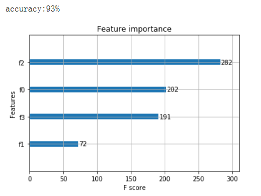
print( 'accuracy:%2.f%%' %(accuracy*100))
# 显示重要特征
plot_importance(model)
plt.show()
2. 回归
import xgboost as xgb
from xgboost import plot_importance
from matplotlib import pyplot as plt
from sklearn.model_selection import train_test_split
from sklearn.datasets import load_boston
# 导入数据集
boston = load_boston()
X ,y = boston.data,boston.target
# Xgboost训练过程
X_train,X_test,y_train,y_test = train_test_split(X,y,test_size=0.2,random_state=0)
model = xgb.XGBRegressor(max_depth=5,learning_rate=0.1,n_estimators=160,silent=True,objective='reg:gamma')
model.fit(X_train,y_train)
# 对测试集进行预测
ans = model.predict(X_test)
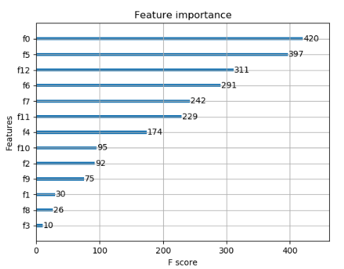
# 显示重要特征
plot_importance(model)
plt.show()
3.3 参数调优的一般方法
调参步骤:
1,选择较高的学习速率(learning rate)。一般情况下,学习速率的值为0.1.但是,对于不同的问题,理想的学习速率有时候会在0.05~0.3之间波动。选择对应于此学习速率的理想决策树数量。Xgboost有一个很有用的函数“cv”,这个函数可以在每一次迭代中使用交叉验证,并返回理想的决策树数量。
2,对于给定的学习速率和决策树数量,进行决策树特定参数调优(max_depth , min_child_weight , gamma , subsample,colsample_bytree)在确定一棵树的过程中,我们可以选择不同的参数。
3,Xgboost的正则化参数的调优。(lambda , alpha)。这些参数可以降低模型的复杂度,从而提高模型的表现。
4,降低学习速率,确定理想参数。
具体调参步骤请看接下来的这个实例
二、XGBOOST实例(分类+调参)
应用XGBoost做一个简单的二分类问题:
用到的数据:https://github.com/tangg9646/file_share/blob/master/pima-indians-diabetes.csv
jupyter格式的文件一并上传在此仓库中
预测待测样本是否会在5年内患糖尿病
数据前8列为特征,最后一列为是否患糖尿病(0 1)
第一部分:默认的xgboost配置
1.导入必须的包
import pandas as pd
import numpy as np
from numpy import loadtxt
from xgboost import XGBClassifier
from sklearn.model_selection import train_test_split
from sklearn.metrics import accuracy_score
from sklearn.model_selection import cross_val_score
后续调参会用到这个函数来比较调参的效果
# 查看训练出来的模型(完成fit 步骤之后)
#在训练集  测试集  上的交叉验证成绩

def cv_score_train_test(model):
    num_cv = 5
    score_list = ["neg_log_loss","accuracy","f1", "roc_auc"]
    train_scores = []
    test_scores = []
    for score in score_list:
        train_scores.append(cross_val_score(model, X_train, y_train, cv=num_cv, scoring=score).mean())
        test_scores.append(cross_val_score(model, X_test, y_test, cv=num_cv, scoring=score).mean())
    scores = np.array((train_scores + test_scores)).reshape(2, -1)
    scores_df = pd.DataFrame(scores, index=['Train', 'Test'], columns=score_list)
    print(scores_df)
2. 数据基本处理
分出变量和标签
dataset = loadtxt('pima-indians-diabetes.csv', delimiter=",")

X = dataset[:,0:8] #左开右闭
Y = dataset[:,8]
将数据分为训练集和测试集
测试集用来预测,训练集用来学习模型
seed = 7
test_size = 0.33
X_train, X_test, y_train, y_test = train_test_split(X, Y, test_size=test_size, random_state=seed)
3. 使用XGBOOST封转好的分类器
全部使用默认参数
直接用XGBClassifier 建立模型
xgb_clf1 = XGBClassifier()
xgb_clf1.fit(X_train, y_train)
XGBClassifier(base_score=0.5, booster='gbtree', colsample_bylevel=1,
       colsample_bynode=1, colsample_bytree=1, gamma=0, learning_rate=0.1,
       max_delta_step=0, max_depth=3, min_child_weight=1, missing=None,
       n_estimators=100, n_jobs=1, nthread=None,
       objective='binary:logistic', random_state=0, reg_alpha=0,
       reg_lambda=1, scale_pos_weight=1, seed=None, silent=None,
       subsample=1, verbosity=1)
4. 进行预测
对测试集进行预测,并将预测的概率值,使用round函数转化为0 1 值
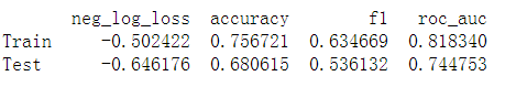
cv_score_train_test(xgb_clf1)
       neg_log_loss  accuracy        f1   roc_auc
Train     -0.502422  0.756721  0.634669  0.818340
Test      -0.646176  0.680615  0.536132  0.744753
不使用封装的函数,单独查看xgboost在测试集上的成绩
y_probablity_pred = xgb_clf1.predict(X_test)
y_predictions = [round(value) for value in y_probablity_pred]
查看在测试集上的预测精度
accuracy = accuracy_score(y_test, y_predictions)
print("Accuracy: %.2f%%" % (accuracy * 100.0))
Accuracy: 77.95%
5. 监控模型的表现
xgboost 可以在模型训练时,评价模型在测试集上的表现,也可以输出每一步的分数
但是需要指定测试集,early_stopping,评价指标
xgb_clf2 = XGBClassifier(
    learning_rate =0.01,
    n_estimators=1000,
    max_depth=5,
    min_child_weight=1,
    gamma=0,
    subsample=0.8,
    colsample_bytree=0.8,
    objective= 'binary:logistic',
    nthread=4,
    scale_pos_weight=1,
    seed=27
)

eval_set = [(X_test, y_test)]
xgb_clf2.fit(
    X_train, y_train,
    early_stopping_rounds=50,
#     eval_metric="logloss",
    eval_metric=["auc", "logloss"],
    eval_set=eval_set,
    verbose=50)
[0]	validation_0-auc:0.716217	validation_0-logloss:0.690588
Multiple eval metrics have been passed: 'validation_0-logloss' will be used for early stopping.

Will train until validation_0-logloss hasn't improved in 50 rounds.
[50]	validation_0-auc:0.833065	validation_0-logloss:0.584058
[100]	validation_0-auc:0.833602	validation_0-logloss:0.532183
[150]	validation_0-auc:0.835749	validation_0-logloss:0.505183
[200]	validation_0-auc:0.832528	validation_0-logloss:0.492587
[250]	validation_0-auc:0.832394	validation_0-logloss:0.485973
[300]	validation_0-auc:0.830784	validation_0-logloss:0.484974
Stopping. Best iteration:
[282]	validation_0-auc:0.831119	validation_0-logloss:0.484596
XGBClassifier(base_score=0.5, booster='gbtree', colsample_bylevel=1,
       colsample_bynode=1, colsample_bytree=0.8, gamma=0,
       learning_rate=0.01, max_delta_step=0, max_depth=5,
       min_child_weight=1, missing=None, n_estimators=1000, n_jobs=1,
       nthread=4, objective='binary:logistic', random_state=0, reg_alpha=0,
       reg_lambda=1, scale_pos_weight=1, seed=27, silent=None,
       subsample=0.8, verbosity=1)
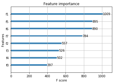
6. 查看特征的重要度
gradient boosting 还有一个优点是可以给出训练好的模型的特征重要性
需要引入XGBOOST中的两个类
from xgboost import plot_importance
import matplotlib.pyplot as plt

# 只需要在模型拟合fit完成之后加入
plot_importance(xgb_clf2)
plt.show()
第二部分:XGBOOST参数调优
XGBOOST参数调优
from sklearn.model_selection import GridSearchCV
from sklearn.model_selection import StratifiedKFold
1. 学习率,估计器数目
#搜索学习率和估计器数目
#其他参数设置为默认值
model1_1 = XGBClassifier(
    max_depth=5,
    min_child_weight=1,
    gamma=0,
    subsample=0.8,
    colsample_bytree=0.8,
    objective= 'binary:logistic',
    nthread=4,
    scale_pos_weight=1,
    seed=27)

#网格搜索参数列表
learning_rate = [ 0.001, 0.01, 0.1, 0.2]
n_estimators = [100, 200, 300, 500, 1000]
param1 = dict(learning_rate=learning_rate, n_estimators=n_estimators)

kfold = StratifiedKFold(n_splits=5, shuffle=True, random_state=7)

#网格搜索类,要求的param_grid参数,必须是字典,或者字典构成的列表
#scoring 参数根据实际情况设定,roc_auc 或者 neg_log_loss
grid_search = GridSearchCV(model1_1, param_grid=param1, scoring="neg_log_loss", n_jobs=-1, cv=kfold, verbose=1)
# grid_search = GridSearchCV(model1_1, param_grid=param1, scoring="roc_auc", n_jobs=-1, cv=kfold, verbose=1)
grid_result = grid_search.fit(X_train, y_train)

print("Best: %f using %s" % (grid_result.best_score_, grid_result.best_params_))
Best: -0.479729 using {'learning_rate': 0.01, 'n_estimators': 300}
设置学习率为上述搜索到的学习率的值,具体查看最优化的 估计其数目 是多少
这一步也可以不要,直接使用上述的最好n_estimators
model1_2 = XGBClassifier(
    learning_rate =0.01,
    n_estimators=400,
    max_depth=5,
    min_child_weight=1,
    gamma=0,
    subsample=0.8,
    colsample_bytree=0.8,
    objective= 'binary:logistic',
    nthread=4,
    scale_pos_weight=1,
    seed=27
)

eval_set = [(X_test, y_test)]
model1_2.fit(
    X_train, y_train,
    early_stopping_rounds=100,
    eval_metric="logloss",
#     eval_metric="auc",
    eval_set=eval_set,
    verbose=50)
#verbose是指,每隔50个estimator才打印一次成绩
[0]	validation_0-logloss:0.690588
Will train until validation_0-logloss hasn't improved in 100 rounds.
[50]	validation_0-logloss:0.584058
[100]	validation_0-logloss:0.532183
[150]	validation_0-logloss:0.505183
[200]	validation_0-logloss:0.492587
[250]	validation_0-logloss:0.485973
[300]	validation_0-logloss:0.484974
[350]	validation_0-logloss:0.486333
Stopping. Best iteration:
[282]	validation_0-logloss:0.484596


XGBClassifier(base_score=0.5, booster='gbtree', colsample_bylevel=1,
       colsample_bynode=1, colsample_bytree=0.8, gamma=0,
       learning_rate=0.01, max_delta_step=0, max_depth=5,
       min_child_weight=1, missing=None, n_estimators=400, n_jobs=1,
       nthread=4, objective='binary:logistic', random_state=0, reg_alpha=0,
       reg_lambda=1, scale_pos_weight=1, seed=27, silent=None,
       subsample=0.8, verbosity=1)
查看训练出来的模型
在训练集 测试集 上的交叉验证成绩
cv_score_train_test(model1_2)
       neg_log_loss  accuracy        f1   roc_auc
Train      -0.49006  0.764489  0.641571  0.819106
Test       -0.55298  0.692769  0.550016  0.779069
结论
- 最佳学习率 0.01
- 估计其数目 300(282)
**如果scoring参数设置为aoc, **
那么n_estimator=50即可在测试集上获得比较好的成绩
如果scoring设置为neg_log_loss
那么需要设置n_estimator需要设置为300左右
2. max_depth 和 min_child_weight
#搜索学习率和估计器数目
#其他参数设置为默认值
model2 = XGBClassifier(
    learning_rate=0.01,
    n_estimators=300,
    gamma=0,
    subsample=0.8,
    colsample_bytree=0.8,
    objective= 'binary:logistic',
    nthread=4,
    scale_pos_weight=1,
    seed=27)

max_depth = [ i for i in range(1, 6)]
min_child_weight = [i for i in range(4, 8)]
param2 = dict(max_depth=max_depth, min_child_weight=min_child_weight)

kfold = StratifiedKFold(n_splits=5, shuffle=True, random_state=7)

#网格搜索类,要求的param_grid参数,必须是字典,或者字典构成的列表
grid_search = GridSearchCV(model2, param_grid=param2, scoring="neg_log_loss", n_jobs=-1, cv=kfold, verbose=1)
grid_result = grid_search.fit(X_train, y_train)

print("Best: %f using %s" % (grid_result.best_score_, grid_result.best_params_))
Best: -0.471508 using {'max_depth': 3, 'min_child_weight': 5}
查看模型在训练集、测试集上的交叉验证成绩
cv_score_train_test(grid_search.best_estimator_)
       neg_log_loss  accuracy        f1   roc_auc
Train     -0.475166  0.758758  0.614573  0.830570
Test      -0.521323  0.751385  0.633099  0.803339
结论:
- 'max_depth': 3
- 'min_child_weight': 5
3. gamma参数调优
model3 = XGBClassifier(
    learning_rate=0.01,
    n_estimators=300,
    max_depth=3,
    min_child_weight=5,
    subsample=0.8,
    colsample_bytree=0.8,
    objective= 'binary:logistic',
    nthread=4,
    scale_pos_weight=1,
    seed=27)

gamma = [ i/10.0 for i in range(5, 12)]
param3 = dict(gamma=gamma)

kfold = StratifiedKFold(n_splits=5, shuffle=True, random_state=7)

#网格搜索类,要求的param_grid参数,必须是字典,或者字典构成的列表
grid_search = GridSearchCV(model3, param_grid=param3, scoring="neg_log_loss", n_jobs=-1, cv=kfold, verbose=1)
grid_result = grid_search.fit(X_train, y_train)

print("Best: %f using %s" % (grid_result.best_score_, grid_result.best_params_))
Fitting 5 folds for each of 7 candidates, totalling 35 fits
Best: -0.471190 using {'gamma': 0.7}
# 查看模型在训练集、测试集上的交叉验证成绩
cv_score_train_test(grid_search.best_estimator_)
       neg_log_loss  accuracy        f1   roc_auc
Train     -0.475537  0.758758  0.614573  0.829718
Test      -0.520716  0.747385  0.630400  0.803452
4.subsample 和 colsample_bytree 参数
model4 = XGBClassifier(
    learning_rate=0.01,
    n_estimators=300,
    max_depth=4,
    min_child_weight=4,
    gamma=0.7,
    objective= 'binary:logistic',
    nthread=4,
    scale_pos_weight=1,
    seed=27)

subsample = [ i/10.0 for i in range(6, 10)]
colsample_bytree  =  [ i/10.0 for i in range(6, 10)]
param4 = dict(subsample=subsample, colsample_bytree=colsample_bytree)

kfold = StratifiedKFold(n_splits=5, shuffle=True, random_state=7)

#网格搜索类,要求的param_grid参数,必须是字典,或者字典构成的列表
grid_search = GridSearchCV(model4, param_grid=param4, scoring="neg_log_loss", n_jobs=-1, cv=kfold, verbose=1)
grid_result = grid_search.fit(X, Y)

print("Best: %f using %s" % (grid_result.best_score_, grid_result.best_params_))
Best: -0.473702 using {'colsample_bytree': 0.7, 'subsample': 0.8}
再次细化上述两个参数
colsample_bytree  =  [ i/100.0 for i in range(65,90,5)]
subsample = [ i/100.0 for i in range(55,95,5)]
param4_2 = dict(subsample=subsample, colsample_bytree=colsample_bytree)

grid_search = GridSearchCV(model4, param_grid=param4_2, scoring="neg_log_loss", n_jobs=-1, cv=kfold, verbose=1)
grid_result = grid_search.fit(X, Y)

print("Best: %f using %s" % (grid_result.best_score_, grid_result.best_params_))
Best: -0.473702 using {'colsample_bytree': 0.65, 'subsample': 0.8}
结论
- 'colsample_bytree': 0.65,
- 'subsample': 0.8
5. 正则化参数调优
model5 = XGBClassifier(
    learning_rate=0.01,
    n_estimators=300,
    max_depth=4,
    min_child_weight=4,
    gamma=0.7,
    subsample=0.8,
    colsample_bytree=0.65,
    objective= 'binary:logistic',
    nthread=4,
    scale_pos_weight=1,
    seed=27)

reg_alpha = [1e-5, 1e-2, 0.1, 1, 100]
reg_lambda  =  [1e-5, 1e-2, 0.1, 1, 100]
param5 = dict(reg_alpha=reg_alpha, reg_lambda=reg_lambda)

kfold = StratifiedKFold(n_splits=5, shuffle=True, random_state=7)

#网格搜索类,要求的param_grid参数,必须是字典,或者字典构成的列表
grid_search = GridSearchCV(model5, param_grid=param5, scoring="neg_log_loss", n_jobs=-1, cv=kfold, verbose=1)
grid_result = grid_search.fit(X, Y)

print("Best: %f using %s" % (grid_result.best_score_, grid_result.best_params_))
Best: -0.473605 using {'reg_alpha': 0.01, 'reg_lambda': 1}
再次细化上述参数
reg_alpha = [1e-3, 1e-2, 0.1]
reg_lambda  =  [0.1, 1, 10]
param5_2 = dict(reg_alpha=reg_alpha, reg_lambda=reg_lambda)

grid_search = GridSearchCV(model5, param_grid=param5_2, scoring="neg_log_loss", n_jobs=-1, cv=kfold, verbose=1)
grid_result = grid_search.fit(X, Y)

print("Best: %f using %s" % (grid_result.best_score_, grid_result.best_params_))
Best: -0.473605 using {'reg_alpha': 0.01, 'reg_lambda': 1}
结论:
- 'reg_alpha': 0.01,
- 'reg_lambda': 1
6. 再次降低学习速率
model6 = XGBClassifier(
    n_estimators=300,
    max_depth=4,
    min_child_weight=4,
    gamma=0.7,
    subsample=0.8,
    colsample_bytree=0.65,
    reg_alpha=0.01,
    reg_lambda=1,
    objective= 'binary:logistic',
    nthread=4,
    scale_pos_weight=1,
    seed=27)

learning_rate = [0.001, 0.01, 0.1, 1]

param6 = dict(learning_rate=learning_rate)

kfold = StratifiedKFold(n_splits=5, shuffle=True, random_state=7)

#网格搜索类,要求的param_grid参数,必须是字典,或者字典构成的列表
grid_search = GridSearchCV(model6, param_grid=param6, scoring="neg_log_loss", n_jobs=-1, cv=kfold, verbose=1)
grid_result = grid_search.fit(X, Y)

print("Best: %f using %s" % (grid_result.best_score_, grid_result.best_params_))
Best: -0.473605 using {'learning_rate': 0.01}
结论
学习率=0.01确实是最好的
7. 完成所有调参
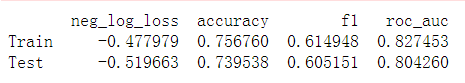
cv_score_train_test(grid_search.best_estimator_)
       neg_log_loss  accuracy        f1   roc_auc
Train     -0.477979  0.756760  0.614948  0.827453
Test      -0.519663  0.739538  0.605151  0.804260
xbg_clf1 model6 模型效果对比