拓端数据tecdat|R语言分段线性回归分析预测车辆的制动距离

原文链接： http://tecdat.cn/?p=21557

分段回归( piecewise regression )，顾名思义，回归式是“分段”拟合的。其灵活用于响应变量随自变量值的改变而存在多种响应状态的情况，二者间难以通过一种回归模型预测或解释时，不妨根据响应状态找到合适的断点位置，然后将自变量划分为有限的区间，并在不同区间内分别构建回归描述二者关系。 分段回归最简单最常见的类型就是分段线性回归( piecewise linear regression )，即各分段内的局部回归均为线性回归。
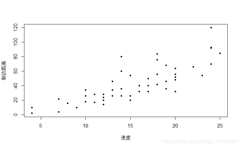
本文我们试图预测车辆的制动距离，同时考虑到车辆的速度。

1.  
   > summary(reg)
2.  
    
3.  
   Call:
4.  
    
5.  
   Residuals:
6.  
   Min 1Q Median 3Q Max
7.  
   -29.069 -9.525 -2.272 9.215 43.201
8.  
    
9.  
   Coefficients:
10.  
    Estimate Std. Error t value Pr(>|t|)
11.  
    (Intercept) -17.5791 6.7584 -2.601 0.0123 *
12.  
    speed 3.9324 0.4155 9.464 1.49e-12 ***
13.  
    ---
14.  
    Signif. codes: 0 ‘***’ 0.001 ‘**’ 0.01 ‘*’ 0.05 ‘.’ 0.1 ‘ ’ 1
15.  
     
16.  
    Residual standard error: 15.38 on 48 degrees of freedom
17.  
    Multiple R-squared: 0.6511, Adjusted R-squared: 0.6438
18.  
    F-statistic: 89.57 on 1 and 48 DF, p-value: 1.49e-12

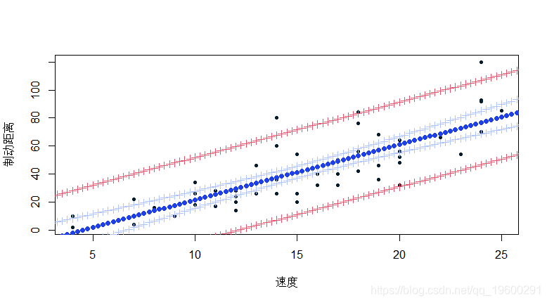
要手动进行多个预测，可以使用以下代码（循环允许对多个值进行预测）

1.  
   for(x in seq(3,30)){
2.  
    
3.  
   + Yx=b0+b1*x
4.  
   + V=vcov(reg)
5.  
   + IC1=Yx+c(-1,+1)*1.96*sqrt(Vx)
6.  
   + s=summary(reg)$sigma
7.  
   + IC2=Yx+c(-1,+1)*1.96*s

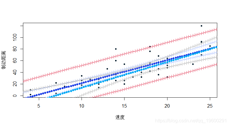
然后在一个随机选择的20个观测值的基础上进行线性回归。

lm(dist~speed,data=cars[I,])

目的是使观测值的数量对回归质量的影响可视化。

1.  
    
2.  
   Residuals:
3.  
   Min 1Q Median 3Q Max
4.  
   -23.529 -7.998 -5.394 11.634 39.348
5.  
    
6.  
   Coefficients:
7.  
   Estimate Std. Error t value Pr(>|t|)
8.  
   (Intercept) -20.7408 9.4639 -2.192 0.0418 *
9.  
   speed 4.2247 0.6129 6.893 1.91e-06 ***
10.  
    ---
11.  
    Signif. codes: 0 ‘***’ 0.001 ‘**’ 0.01 ‘*’ 0.05 ‘.’ 0.1 ‘ ’ 1
12.  
     
13.  
    Residual standard error: 16.62 on 18 degrees of freedom
14.  
    Multiple R-squared: 0.7252, Adjusted R-squared: 0.71
15.  
    F-statistic: 47.51 on 1 and 18 DF, p-value: 1.91e-06
16.  
     
17.  
    > for(x in seq(3,30,by=.25)){
18.  
     
19.  
    + Yx=b0+b1*x
20.  
    + V=vcov(reg)
21.  
    + IC=Yx+c(-1,+1)*1.96*sqrt(Vx)
22.  
    + points(x,Yx,pch=19

可以使用R函数进行预测，具有置信区间

1.  
   fit lwr upr
2.  
   1 42.62976 34.75450 50.50502
3.  
   2 84.87677 68.92746 100.82607
4.  
   > predict(reg,
5.  
   fit lwr upr
6.  
   1 42.62976 6.836077 78.42344

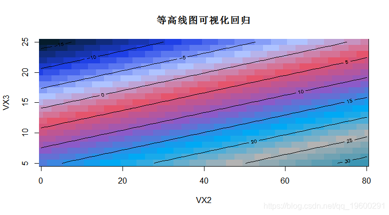
当有多个解释变量时，“可视化”回归就变得更加复杂了

1.  
    
2.  
   > image(VX2,VX3,VY)
3.  
   > contour(VX2,VX3,VY,add=TRUE)

这是一个回归三维曲面图

> persp(VX2,VX3,VY,ticktype=detailed)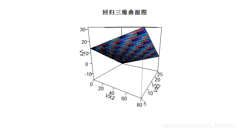

我们将更详细地讨论这一点，但从这个线性模型中可以很容易地进行非线性回归。我们从距离对数的线性模型开始

1.  
    
2.  
   > abline(reg1)

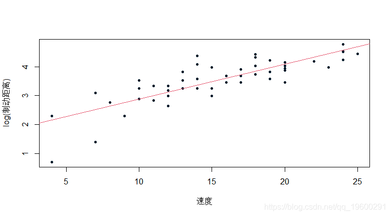
因为我们在这里没有任何关于距离的预测，只是关于它的对数......但我们稍后会讨论它

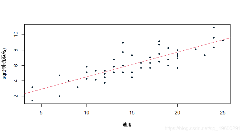
lm(sqrt(dist)~speed,data=cars)

还可以转换解释变量。你可以设置断点(阈值)。我们从一个指示变量开始

1.  
    
2.  
   Residuals:
3.  
   Min 1Q Median 3Q Max
4.  
   -29.472 -9.559 -2.088 7.456 44.412
5.  
    
6.  
   Coefficients:
7.  
   Estimate Std. Error t value Pr(>|t|)
8.  
   (Intercept) -17.2964 6.7709 -2.555 0.0139 *
9.  
   speed 4.3140 0.5762 7.487 1.5e-09 ***
10.  
    speed > s TRUE -7.5116 7.8511 -0.957 0.3436
11.  
    ---
12.  
    Signif. codes: 0 ‘***’ 0.001 ‘**’ 0.01 ‘*’ 0.05 ‘.’ 0.1 ‘ ’ 1
13.  
     
14.  
    Residual standard error: 15.39 on 47 degrees of freedom
15.  
    Multiple R-squared: 0.6577, Adjusted R-squared: 0.6432
16.  
    F-statistic: 45.16 on 2 and 47 DF, p-value: 1.141e-11

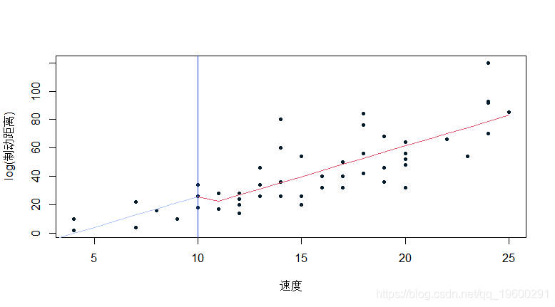
但是你也可以把函数放在一个分段的线性模型里，同时保持连续性。

1.  
    
2.  
   Residuals:
3.  
   Min 1Q Median 3Q Max
4.  
   -29.502 -9.513 -2.413 5.195 45.391
5.  
    
6.  
   Coefficients:
7.  
   Estimate Std. Error t value Pr(>|t|)
8.  
   (Intercept) -7.6519 10.6254 -0.720 0.47500
9.  
   speed 3.0186 0.8627 3.499 0.00103 **
10.  
    speed - s 1.7562 1.4551 1.207 0.23350
11.  
    ---
12.  
    Signif. codes: 0 ‘***’ 0.001 ‘**’ 0.01 ‘*’ 0.05 ‘.’ 0.1 ‘ ’ 1
13.  
     
14.  
    Residual standard error: 15.31 on 47 degrees of freedom
15.  
    Multiple R-squared: 0.6616, Adjusted R-squared: 0.6472
16.  
    F-statistic: 45.94 on 2 and 47 DF, p-value: 8.761e-12

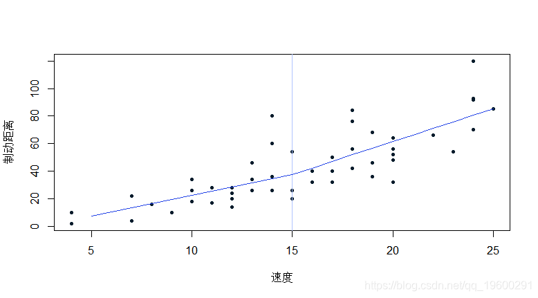
在这里，我们可以想象几个分段

1.  
   posi=function(x) ifelse(x>0,x,0)
2.  
    
3.  
    
4.  
   Coefficients:
5.  
   Estimate Std. Error t value Pr(>|t|)
6.  
   (Intercept) -7.6305 16.2941 -0.468 0.6418
7.  
   speed 3.0630 1.8238 1.679 0.0998 .
8.  
   positive(speed - s1) 0.2087 2.2453 0.093 0.9263
9.  
   positive(speed - s2) 4.2812 2.2843 1.874 0.0673 .
10.  
    ---
11.  
    Signif. codes: 0 ‘***’ 0.001 ‘**’ 0.01 ‘*’ 0.05 ‘.’ 0.1 ‘ ’ 1
12.  
     
13.  
    Residual standard error: 15 on 46 degrees of freedom
14.  
    Multiple R-squared: 0.6821, Adjusted R-squared: 0.6613
15.  
    F-statistic: 32.89 on 3 and 46 DF, p-value: 1.643e-11

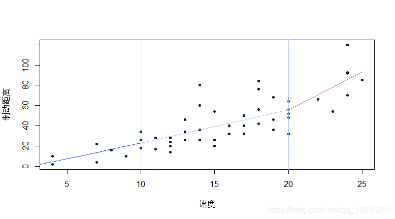
正如目前所看到的，后两个系数的显著性测试并不意味着斜率为零，而是与左侧区域（在两个阈值之前）的斜率显著不同。

---

最受欢迎的见解

1.R语言多元Logistic逻辑回归 应用案例

2.面板平滑转移回归(PSTR)分析案例实现

3.matlab中的偏最小二乘回归（PLSR）和主成分回归（PCR）

4.R语言泊松Poisson回归模型分析案例

5.R语言回归中的Hosmer-Lemeshow拟合优度检验

6.r语言中对LASSO回归，Ridge岭回归和Elastic Net模型实现

7.在R语言中实现Logistic逻辑回归

8.python用线性回归预测股票价格

9.R语言如何在生存分析与Cox回归中计算IDI，NRI指标