频域分析及变换
更多精彩内容请关注微信公众号:听潮庭。
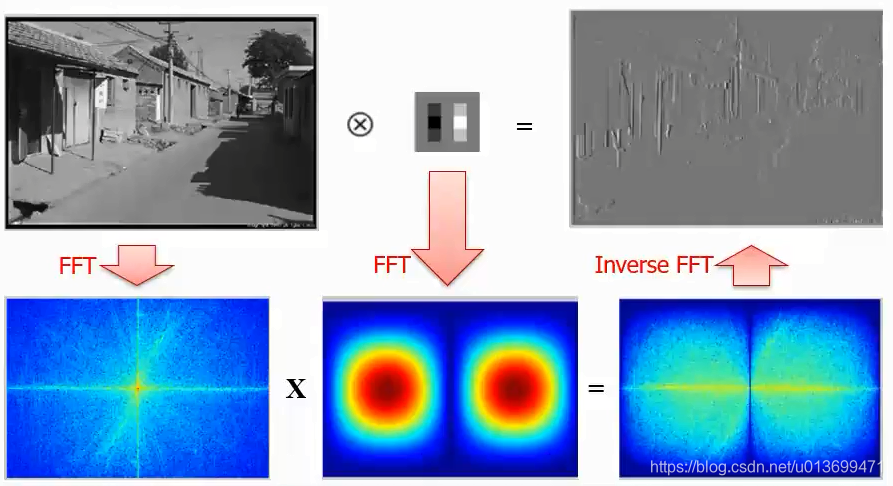
如何让卷积更快:空域卷积=频域卷积
-
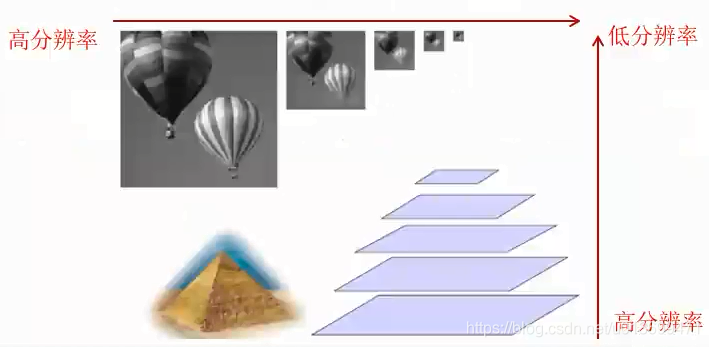
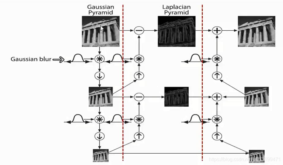
图像金字塔化:先进行图像平滑,再进行降采样,
-
根据降采样率,得到一系列尺寸逐渐减小的图像。
-
操作:n次(高斯卷积->2倍降采样)->n层金字塔
-
目的:捕捉不同尺寸的物体
-
-
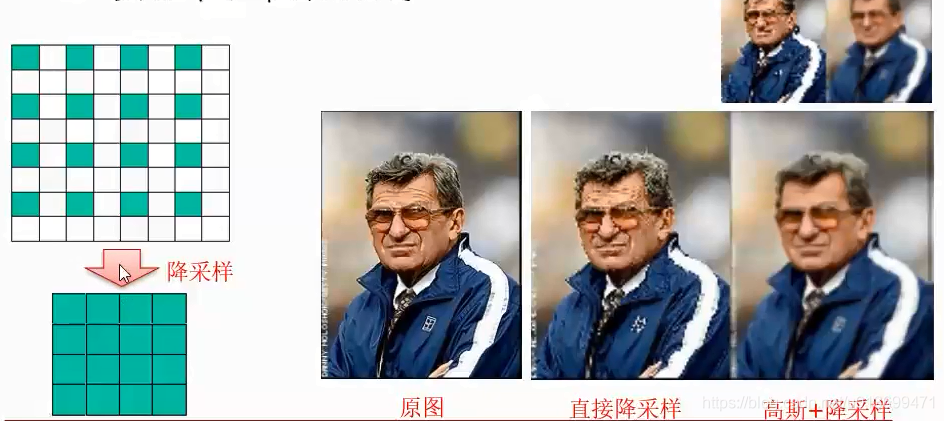
高斯滤波的必要性:直接降采样损失信息
-
高斯金字塔本质上为信号的多尺度表示法
-
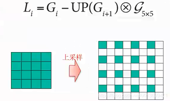
- 高频细节信息在卷积和下采样中丢失
- 保留所有层所丢失的高频信息,用于图像恢复
- 下采样
- 上采样
- 高斯模糊
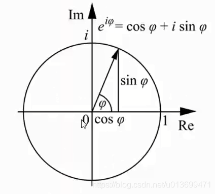
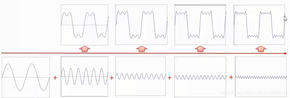
- 一个信号可以由足够多个不同频率和幅值的正余弦波组成
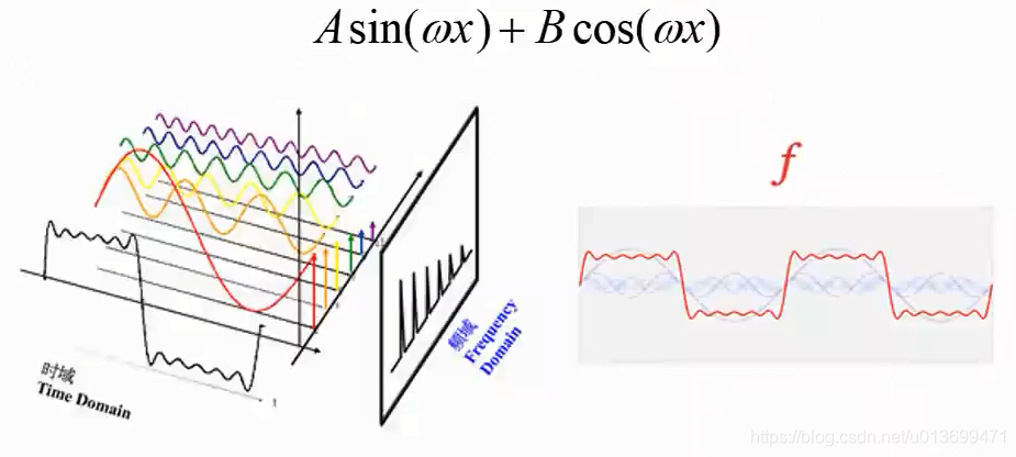
- 信号分解:
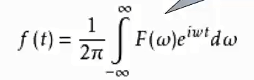
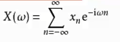
- 傅里叶变换的数学公式:连续变换
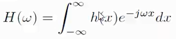
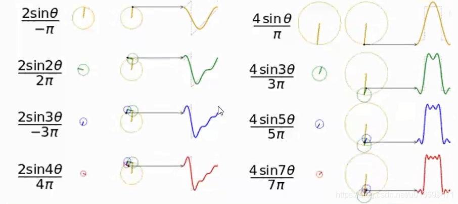
- 欧拉公式
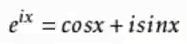

- 欧拉公式描述的是一个随着时间变化,在复平面上做圆周运动的点;
- 傅里叶变换描述的就是一系列这样的点的运动的叠加的效应
- 傅里叶逆变换
-
-
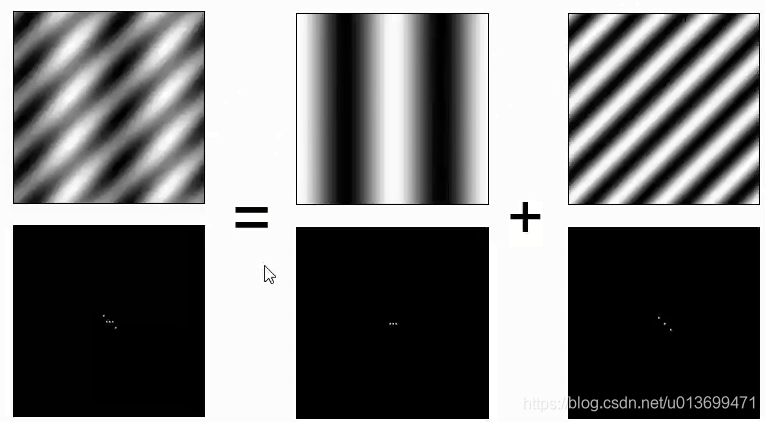
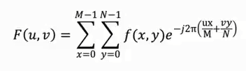
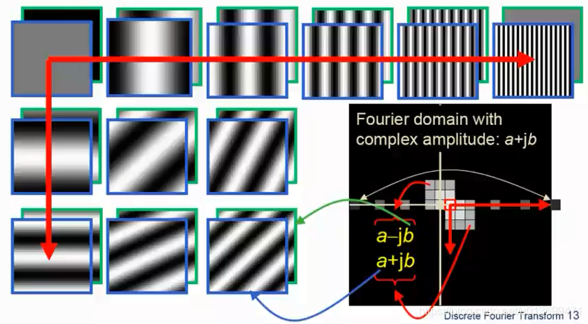
二维离散傅里叶变换:
-
-
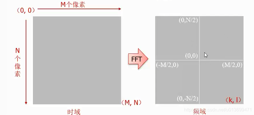
- 2D傅里叶基图片(越靠外的 是条纹越密集的地方)

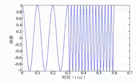
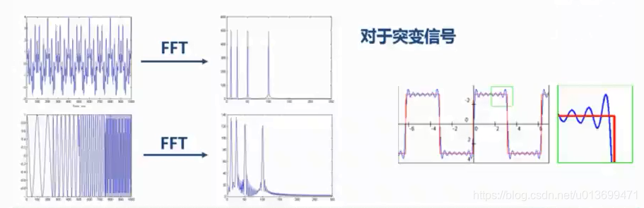
- 关键问题:傅里叶变换假设前提为信号平稳,但实际中信号多数为非平稳信号。
- 缺乏时间和频率的定位功能
- 对于非平稳信号的局限性
- 在时间和频率分辨率上的局限性
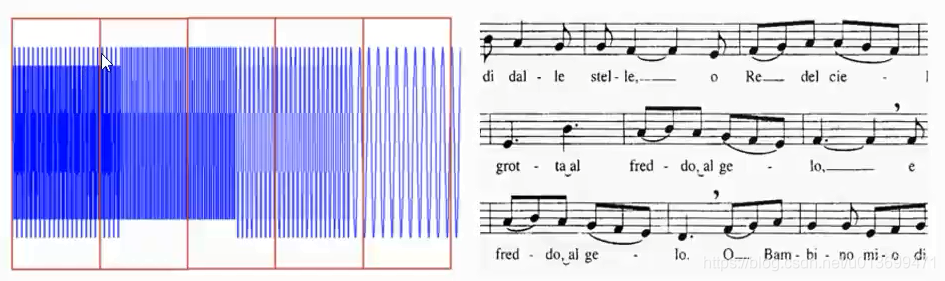
- SIFT(短时傅里叶变换)添加时域信息的方法是设置窗格,认为窗格内的信号是平稳的;
- 然后对窗格内的信号分段进行傅里叶变换;
- 优点是可以获得频域信息的同时可以获得时域信息。
- 缺点是窗格大小很难设置。
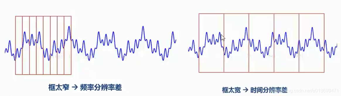
- 短时傅里叶变换的特点:
- 窄窗口时间分辨率高、频率分辨率低;
- 宽窗口时间分辨率低,频率分辨率高;
- 对于时变的非稳态信号,高频适合小窗口。低频适合打窗口
- 但是STFT的窗口是固定的
- 小波变换与STFT思路接近,但小波变换直接把傅里叶变换的基给换了-----将无限长的三角函数基换成了有限长的会衰减的小波基。
- 这样不仅能够获取频率,还可以定位到时间;
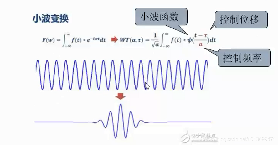
- 所谓的小波函数,是一族函数,需要满足:
- 1、均值为0;
- 在时域和频域都局部化,不蔓延到整个坐标轴
- 满足这两条的函数就是小波(Wavelet)函数,有很多种类,最简单的是Haar小波。
- 小波变换要做的就是将原始信号表示为一组小波基的线性组合,然后通过忽略其中不重要的部分达到数据压缩(即降维)的目的。
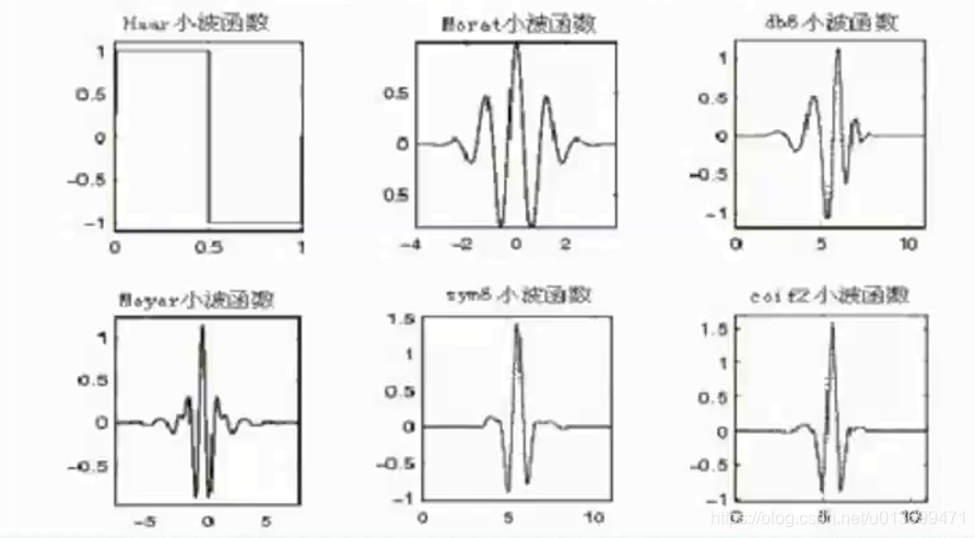
- 常用的小波函数包括:
- Haar系列,Daubechies系列,Moret系列;
- Sym系列,Meyer系列,Coif系列。
-
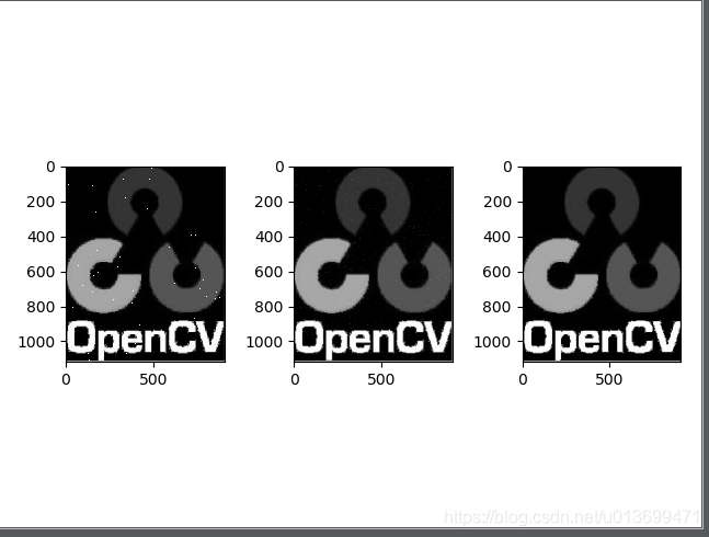
 1 import cv2
 2 import numpy as np
 3 import matplotlib.pyplot as plt
 4
 5 img = cv2.imread('opencv.png',0) #0 直接读为灰度图像
 6 for i in range(2000): #添加点噪声
 7     temp_x = np.random.randint(0,img.shape[0])
 8     temp_y = np.random.randint(0,img.shape[1])
 9     img[temp_x][temp_y] = 255 #在temp_x,temp_y处添加白色噪声(255是白色,0是黑色)
10
11 blur_1 = cv2.GaussianBlur(img,(5,5),0)
12
13 blur_2 = cv2.medianBlur(img,5)
14
15 plt.subplot(1,3,1),plt.imshow(img,'gray')#默认彩色,另一种彩色bgr
16 plt.subplot(1,3,2),plt.imshow(blur_1,'gray')
17 plt.subplot(1,3,3),plt.imshow(blur_2,'gray')
18 plt.show()
-
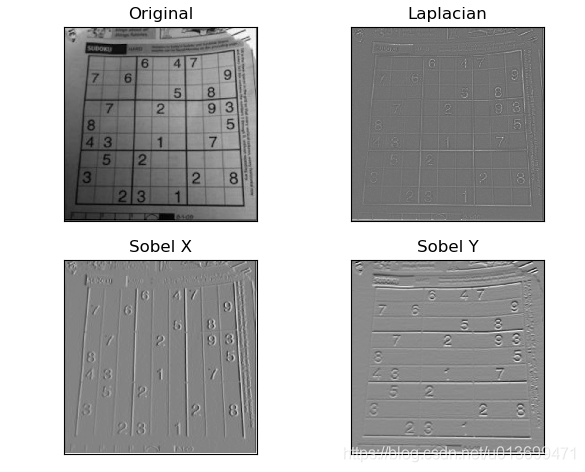
边缘探测
 1 import numpy as np
 2 import cv2 as cv
 3 from matplotlib import pyplot as plt
 4
 5 img = cv.imread('dave.png',0)
 6 laplacian = cv.Laplacian(img,cv.CV_64F)
 7 sobelx = cv.Sobel(img,cv.CV_64F,1,0,ksize=5)
 8 sobely = cv.Sobel(img,cv.CV_64F,0,1,ksize=5)
 9
10 plt.subplot(2,2,1),plt.imshow(img,cmap = 'gray')
11 plt.title('Original'), plt.xticks([]), plt.yticks([])
12
13 plt.subplot(2,2,2),plt.imshow(laplacian,cmap = 'gray')
14 plt.title('Laplacian'), plt.xticks([]), plt.yticks([])
15
16 plt.subplot(2,2,3),plt.imshow(sobelx,cmap = 'gray')
17 plt.title('Sobel X'), plt.xticks([]), plt.yticks([])
18
19 plt.subplot(2,2,4),plt.imshow(sobely,cmap = 'gray')
20 plt.title('Sobel Y'), plt.xticks([]), plt.yticks([])
21 plt.show()
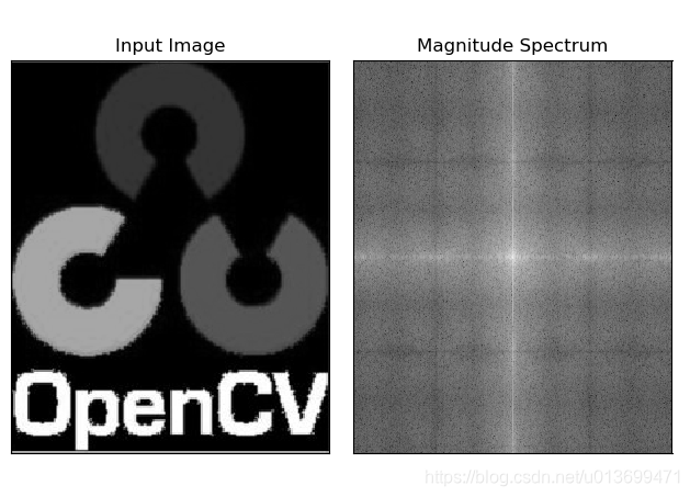
 1 import cv2 as cv
 2 import numpy as np
 3 from matplotlib import pyplot as plt
 4
 5 img = cv.imread('opencv.png',0)
 6 f = np.fft.fft2(img)
 7 fshift = np.fft.fftshift(f)
 8 magnitude_spectrum = 20*np.log(np.abs(fshift))
 9
10 plt.subplot(121),plt.imshow(img, cmap = 'gray')
11 plt.title('Input Image'), plt.xticks([]), plt.yticks([])
12 plt.subplot(122),plt.imshow(magnitude_spectrum, cmap = 'gray')
13 plt.title('Magnitude Spectrum'), plt.xticks([]), plt.yticks([])
14 plt.show()
 1 import cv2
 2 import matplotlib.pyplot as plt
 3
 4 img = cv2.imread('timg.jpg',0) #直接读为灰度图像
 5 res = cv2.equalizeHist(img)
 6
 7 clahe = cv2.createCLAHE(clipLimit=2,tileGridSize=(10,10))
 8 cl1 = clahe.apply(img)
 9
10 plt.subplot(131),plt.imshow(img,'gray')
11 plt.subplot(132),plt.imshow(res,'gray')
12 plt.subplot(133),plt.imshow(cl1,'gray')
13
14 plt.show()
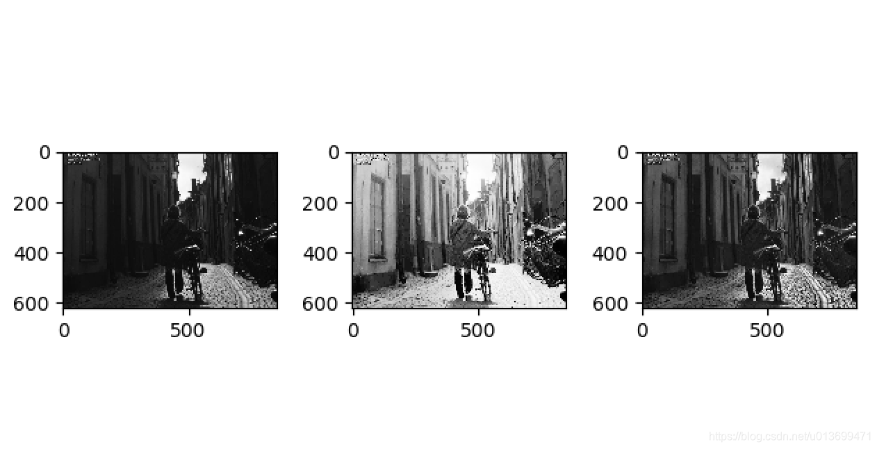
中间是自适应直方图均衡的效果 右边是Clahe