Deep learning：十二(PCA和whitening在二自然图像中的练习)

　　前言:

　　现在来用PCA，PCA Whitening对自然图像进行处理。这些理论知识参考前面的博文：Deep learning：十(PCA和whitening)。而本次试验的数据，步骤，要求等参考网页：http://deeplearning.stanford.edu/wiki/index.php/UFLDL_Tutorial 。实验数据是从自然图像中随机选取10000个12*12的patch，然后对这些patch进行99%的方差保留的PCA计算，最后对这些patch做PCA Whitening和ZCA Whitening，并进行比较。

　　实验环境：matlab2012a

　　实验过程及结果：

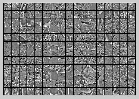
　　随机选取10000个patch，并显示其中204个patch，如下图所示：

 　　

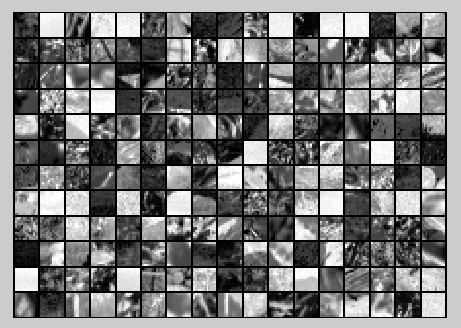
　　然后对这些patch做均值为0化操作得到如下图：

 　　

　　对选取出的patch做PCA变换得到新的样本数据，其新样本数据的协方差矩阵如下图所示：

 　　

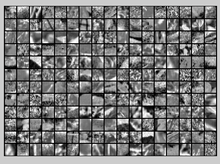
　　保留99%的方差后的PCA还原原始数据，如下所示：

 　　

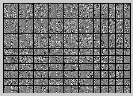
　　PCA Whitening后的图像如下：

 　　

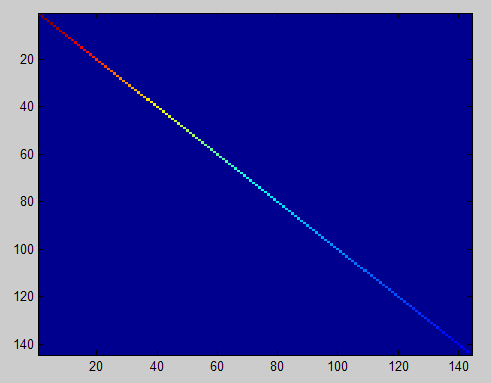
　　此时样本patch的协方差矩阵如下:

 　　

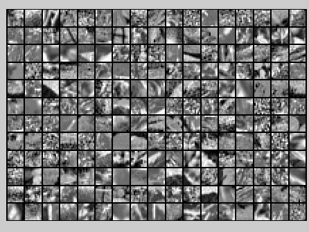
　　ZCA Whitening的结果如下：

 　　

　　实验代码及注释：

%%================================================================
%% Step 0a: Load data
%  Here we provide the code to load natural image data into x.
%  x will be a 144 * 10000 matrix, where the kth column x(:, k) corresponds to
%  the raw image data from the kth 12x12 image patch sampled.
%  You do not need to change the code below.

x = sampleIMAGESRAW();
figure('name','Raw images');
randsel = randi(size(x,2),204,1); % A random selection of samples for visualization
display_network(x(:,randsel));%为什么x有负数还可以显示？

%%================================================================
%% Step 0b: Zero-mean the data (by row)
%  You can make use of the mean and repmat/bsxfun functions.

% -------------------- YOUR CODE HERE -------------------- 
x = x-repmat(mean(x,1),size(x,1),1);%求的是每一列的均值
%x = x-repmat(mean(x,2),1,size(x,2));

%%================================================================
%% Step 1a: Implement PCA to obtain xRot
%  Implement PCA to obtain xRot, the matrix in which the data is expressed
%  with respect to the eigenbasis of sigma, which is the matrix U.


% -------------------- YOUR CODE HERE -------------------- 
xRot = zeros(size(x)); % You need to compute this
[n m] = size(x);
sigma = (1.0/m)*x*x';
[u s v] = svd(sigma);
xRot = u'*x;


%%================================================================
%% Step 1b: Check your implementation of PCA
%  The covariance matrix for the data expressed with respect to the basis U
%  should be a diagonal matrix with non-zero entries only along the main
%  diagonal. We will verify this here.
%  Write code to compute the covariance matrix, covar. 
%  When visualised as an image, you should see a straight line across the
%  diagonal (non-zero entries) against a blue background (zero entries).

% -------------------- YOUR CODE HERE -------------------- 
covar = zeros(size(x, 1)); % You need to compute this
covar = (1./m)*xRot*xRot';

% Visualise the covariance matrix. You should see a line across the
% diagonal against a blue background.
figure('name','Visualisation of covariance matrix');
imagesc(covar);

%%================================================================
%% Step 2: Find k, the number of components to retain
%  Write code to determine k, the number of components to retain in order
%  to retain at least 99% of the variance.

% -------------------- YOUR CODE HERE -------------------- 
k = 0; % Set k accordingly
ss = diag(s);
% for k=1:m
%    if sum(s(1:k))./sum(ss) < 0.99
%        continue;
% end
%其中cumsum(ss)求出的是一个累积向量，也就是说ss向量值的累加值
%并且(cumsum(ss)/sum(ss))<=0.99是一个向量，值为0或者1的向量，为1表示满足那个条件
k = length(ss((cumsum(ss)/sum(ss))<=0.99));

%%================================================================
%% Step 3: Implement PCA with dimension reduction
%  Now that you have found k, you can reduce the dimension of the data by
%  discarding the remaining dimensions. In this way, you can represent the
%  data in k dimensions instead of the original 144, which will save you
%  computational time when running learning algorithms on the reduced
%  representation.
% 
%  Following the dimension reduction, invert the PCA transformation to produce 
%  the matrix xHat, the dimension-reduced data with respect to the original basis.
%  Visualise the data and compare it to the raw data. You will observe that
%  there is little loss due to throwing away the principal components that
%  correspond to dimensions with low variation.

% -------------------- YOUR CODE HERE -------------------- 
xHat = zeros(size(x));  % You need to compute this
xHat = u*[u(:,1:k)'*x;zeros(n-k,m)];

% Visualise the data, and compare it to the raw data
% You should observe that the raw and processed data are of comparable quality.
% For comparison, you may wish to generate a PCA reduced image which
% retains only 90% of the variance.

figure('name',['PCA processed images ',sprintf('(%d / %d dimensions)', k, size(x, 1)),'']);
display_network(xHat(:,randsel));
figure('name','Raw images');
display_network(x(:,randsel));

%%================================================================
%% Step 4a: Implement PCA with whitening and regularisation
%  Implement PCA with whitening and regularisation to produce the matrix
%  xPCAWhite. 

epsilon = 0.1;
xPCAWhite = zeros(size(x));

% -------------------- YOUR CODE HERE -------------------- 
xPCAWhite = diag(1./sqrt(diag(s)+epsilon))*u'*x;
figure('name','PCA whitened images');
display_network(xPCAWhite(:,randsel));

%%================================================================
%% Step 4b: Check your implementation of PCA whitening 
%  Check your implementation of PCA whitening with and without regularisation. 
%  PCA whitening without regularisation results a covariance matrix 
%  that is equal to the identity matrix. PCA whitening with regularisation
%  results in a covariance matrix with diagonal entries starting close to 
%  1 and gradually becoming smaller. We will verify these properties here.
%  Write code to compute the covariance matrix, covar. 
%
%  Without regularisation (set epsilon to 0 or close to 0), 
%  when visualised as an image, you should see a red line across the
%  diagonal (one entries) against a blue background (zero entries).
%  With regularisation, you should see a red line that slowly turns
%  blue across the diagonal, corresponding to the one entries slowly
%  becoming smaller.

% -------------------- YOUR CODE HERE -------------------- 
covar = (1./m)*xPCAWhite*xPCAWhite';

% Visualise the covariance matrix. You should see a red line across the
% diagonal against a blue background.
figure('name','Visualisation of covariance matrix');
imagesc(covar);

%%================================================================
%% Step 5: Implement ZCA whitening
%  Now implement ZCA whitening to produce the matrix xZCAWhite. 
%  Visualise the data and compare it to the raw data. You should observe
%  that whitening results in, among other things, enhanced edges.

xZCAWhite = zeros(size(x));

% -------------------- YOUR CODE HERE -------------------- 
xZCAWhite = u*xPCAWhite;

% Visualise the data, and compare it to the raw data.
% You should observe that the whitened images have enhanced edges.
figure('name','ZCA whitened images');
display_network(xZCAWhite(:,randsel));
figure('name','Raw images');
display_network(x(:,randsel));

　　参考资料:

     Deep learning：十(PCA和whitening)

     http://deeplearning.stanford.edu/wiki/index.php/UFLDL_Tutorial