数据分析常用的python工具和SQL语句

select symbol, "price.*" from stocks :使用正则表达式来指定列查询

select count(*), avg(salary) from emplyee: 聚合函数

select count(distinct col) from stocks:去重后的数目

嵌套查询：

from(select upper(name), salary,deductions["Federal Taxes"] as fed_taxes,round(salary*(1-deductions["Federal Taxes"])) as salary_minus from employees) e select e.name, e.salary_mines,where e.salary_minus>70000;

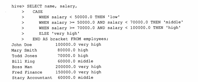
case...when...then...查询

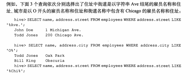
like语句查询：

Rlike语句

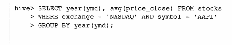
group by 语句

group by 语句通常会和聚合函数一块使用，按照一个或者多个列对结果进行分组，然后对每个分组进行聚合操作。

Hive中的order by 和sort by 的区别：

order by执行的是一个全局排序，也就是说也就是说所有的数据都是通过一个Reducer来排序的，对于大数据集来说，话费很长世间，而sort by是局部排序，在每个Reducer中对数据进行排序，也就是说在每个Reducer中是有序的，但是所有Reducer合起来，就是局部有序。

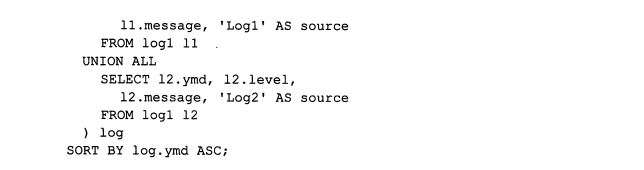
Union all

Union all 可以将2个或者多个表进行合并。但是每一个Union 子查询必须有相同的列，而且每个字段的类型必须是一样的。

下面是hive当中的一些常用函数：

数据函数，集合函数，类型转化函数，日期函数，，条件函数，字符函数，聚合函数，表生成函数。

from_unixtime(bigint unixtime[, string format])：将时间秒值转化为Format格式的时间

例如：from_unixtime(1250111000,"yyyy-MM-dd") 得到2009-03-12

unix_timestamp(string date, string pattern)：将format格式的时间字符串转化为时间戳：

例如：unix_timestamp('2009-03-20 11:30:01') = 1237573801

python工具：

数据预览：

df.head(n); df.info(); df.describe(); df.tail()

df.columns：行名

df.index：列名

train.shape

train.dtypes

pd.concat([train, test],ignore_index=True)

only_western_europe_10 = (reprot_2016_df['地区'] == 'Western Europe') & (reprot_2016_df['排名'] > 10)

df.set_index(['Region', 'Country'])：设置层级索引

数据清洗

log_data.isnull()：是否缺失

log_data[log_data['volume'].notnull()]：取出volume不为空的数据

log_data.fillna(0)：填充缺失数据为0

log_data.dropna()：去掉有缺失数据的记录

log_data.ffill()：以前面的数据填充

log_data.bfill()：以后面的数据填充

data.duplicated()：判断是否重复

data.drop_duplicates()：去除重复数据

map:使用

meat_to_animal = {
'bacon': 'pig',
'pulled pork': 'pig',
'pastrami': 'cow',
'corned beef': 'cow',
'honey ham': 'pig',
'nova lox': 'salmon'
}

lowercased = data['food'].str.lower()
data['animal'] = lowercased.map(meat_to_animal)

或者：

data['food'].map(lambda x: meat_to_animal[x.lower()])

# 将-999替换为空值
data.replace([-999, -1000], np.nan)：将列表里的数替换为nan

split_df = data.str.split('@', expand=True)：str各种函数

pd.merge(staff_df, student_df, how='outer', on='姓名')：合并df，可选择左右内外连接

staff_df['员工姓名'].apply(lambda x: x[0])：apply的使用

report_data.groupby('Region')grouped['Happiness Score'].mean()：后面的聚合函数是对每个分组进行操作的

# 迭代groupby对象
for group, frame in grouped:
mean_score = frame['Happiness Score'].mean()
max_score = frame['Happiness Score'].max()
min_score = frame['Happiness Score'].min()

grouped.agg({'Happiness Score': np.mean, 'Happiness Rank': np.max})：分组的聚合函数

grouped['Happiness Score'].agg([mean, amax, amin, std])：分组的聚合函数

绘图：matplotlib 和 seaborn工具：

%matplotlib notebook：魔法命令

plt.style.available：可用的绘图样式

plt.style.use('seaborn-colorblind')：设置绘图样式

df.plot()：分别以每一列为纵轴，索引为横轴，画曲线图，并以图例区别开来

df.plot('A', 'B', kind='scatter')：指定A为横轴，B为纵轴

df.plot(kind='box')：kind可以为hist，kde

pd.plotting.scatter_matrix(iris)：散点距阵，查看各个特征之间的相关性

sns.pairplot(iris, hue='Name', diag_kind='kde')：查看各个特征之间的相关性

 特征工程：

归一化：

scaler = MinMaxScaler()
X_train_scaled = scaler.fit_transform(X_train)
X_test_scaled = scaler.transform(X_test)

标签编码和独热编码：

首先训练集：

# 在训练集上进行编码操作
label_enc1 = LabelEncoder() # 首先将male, female用数字编码
one_hot_enc = OneHotEncoder() # 将数字编码转换为独热编码

label_enc2 = LabelEncoder() # 将low, middle, high用数字编码

tr_feat1_tmp = label_enc1.fit_transform(X_train[:, 0]).reshape(-1, 1) # reshape(-1, 1)保证为一维列向量
tr_feat1 = one_hot_enc.fit_transform(tr_feat1_tmp)
tr_feat1 = tr_feat1.todense()

tr_feat2 = label_enc2.fit_transform(X_train[:, 1]).reshape(-1, 1)

X_train_enc = np.hstack((tr_feat1, tr_feat2))

然后再测试集上：

te_feat1_tmp = label_enc1.transform(X_test[:, 0]).reshape(-1, 1) # reshape(-1, 1)保证为一维列向量
te_feat1 = one_hot_enc.transform(te_feat1_tmp)
te_feat1 = te_feat1.todense()

te_feat2 = label_enc2.transform(X_test[:, 1]).reshape(-1, 1)

X_test_enc = np.hstack((te_feat1, te_feat2))

模型持久化：

# 保存模型到硬盘
model_path2 = './trained_model2.pkl'
joblib.dump(best_model, model_path2)

model = joblib.load(model_path2) 

 日期特征处理：

train['created'] = pd.to_datetime(train['created'])
train['date'] = train['created'].dt.date
train["year"] = train["created"].dt.year
train['month'] = train['created'].dt.month
train['day'] = train['created'].dt.day

data[v].value_counts()：列举不同的取值，以及每种取值的次数

data.drop(['Loan_Amount_Submitted','Loan_Tenure_Submitted'],axis=1,inplace=True)：删除某列

df_train_origin[['temp','weather','windspeed','day', 'month', 'hour','count']].corr()：相关性

pd.get_dummies(all_df['MSSubClass'], prefix='MSSubClass')：独热编码一键搞定

all_dummy_df.isnull().sum().sort_values(ascending=False)：统计各个字段的空值数目

all_dummy_df.isnull().sum().sum()：各个字段的总空值数

合并之后的数据重新分开：

dummy_train_df = all_dummy_df.loc[train_df.index]
dummy_test_df = all_dummy_df.loc[test_df.index]

df.unstack() 行索引→列索引

df.stack() 列索引→行索引