吴裕雄--天生自然python机器学习：使用K-近邻算法改进约会网站的配对效果

在约会网站使用K-近邻算法

 准备数据：从文本文件中解析数据

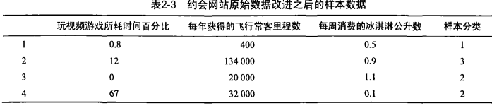
海伦收集约会数据巳经有了一段时间，她把这些数据存放在文本文件(1如1^及抓 比加 中，每
个样本数据占据一行，总共有1000行。海伦的样本主要包含以下3种特征：

每年获得的飞行常客里程数

玩视频游戏所耗时间百分比

每周消费的冰淇淋公升数

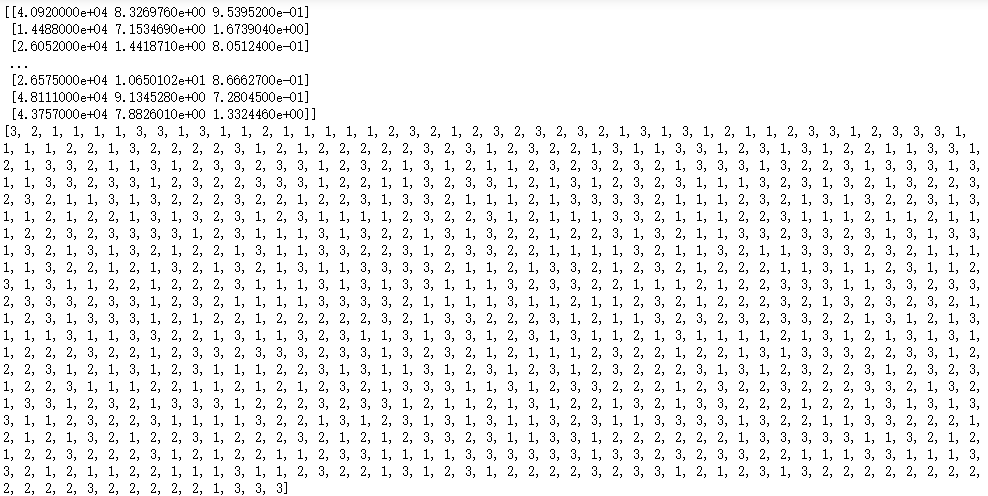
将文本记录到转换NumPy的解析程序

import operator
from numpy import *
from os import listdir

def file2matrix(filename):
    fr = open(filename)
    numberOfLines = len(fr.readlines())         #get the number of lines in the file
    returnMat = zeros((numberOfLines,3))        #prepare matrix to return
    classLabelVector = []                       #prepare labels return   
    fr = open(filename)
    index = 0
    for line in fr.readlines():
        line = line.strip()
        listFromLine = line.split('	')
        returnMat[index,:] = listFromLine[0:3]
        classLabelVector.append(int(listFromLine[-1]))
        index += 1
    return returnMat,classLabelVector

returnMat,classLabelVector = file2matrix('F:\machinelearninginaction\Ch02\datingTestSet2.txt')
print(returnMat)
print(classLabelVector)

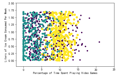
现在已经从文本文件中导人了数据，并将其格式化为想要的格式，接着我们需要了解数据的
真实含义。当然我们可以直接浏览文本文件，但是这种方法非常不友好，一般来说，我们会采用
图形化的方式直观地展示数据。下面就用?^1!(瓜工具来图形化展示数据内容，以便辨识出一些数
据模式。

import matplotlib
import matplotlib.pyplot as plt

from numpy import *

fig = plt.figure()
ax = fig.add_subplot(111)
datingDataMat,datingLabels = file2matrix('F:\machinelearninginaction\Ch02\datingTestSet2.txt')
#ax.scatter(datingDataMat[:,1], datingDataMat[:,2])
ax.scatter(datingDataMat[:,1], datingDataMat[:,2], 15.0*array(datingLabels), 15.0*array(datingLabels))
ax.axis([-2,25,-0.2,2.0])
plt.xlabel('Percentage of Time Spent Playing Video Games')
plt.ylabel('Liters of Ice Cream Consumed Per Week')
plt.show()

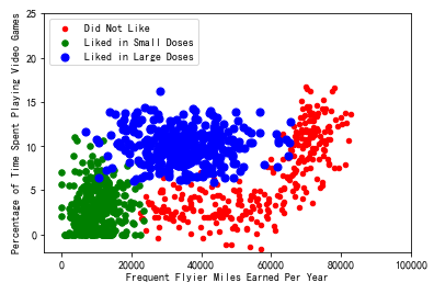
import matplotlib
import matplotlib.pyplot as plt

from numpy import *
from matplotlib.patches import Rectangle


n = 1000 #number of points to create
xcord1 = []; ycord1 = []
xcord2 = []; ycord2 = []
xcord3 = []; ycord3 = []
markers =[]
colors =[]
fw = open('E:\testSet.txt','w')
for i in range(n):
    [r0,r1] = random.standard_normal(2)
    myClass = random.uniform(0,1)
    if (myClass <= 0.16):
        fFlyer = random.uniform(22000, 60000)
        tats = 3 + 1.6*r1
        markers.append(20)
        colors.append(2.1)
        classLabel = 1 #'didntLike'
        xcord1.append(fFlyer); ycord1.append(tats)
    elif ((myClass > 0.16) and (myClass <= 0.33)):
        fFlyer = 6000*r0 + 70000
        tats = 10 + 3*r1 + 2*r0
        markers.append(20)
        colors.append(1.1)
        classLabel = 1 #'didntLike'
        if (tats < 0): tats =0
        if (fFlyer < 0): fFlyer =0
        xcord1.append(fFlyer); ycord1.append(tats)
    elif ((myClass > 0.33) and (myClass <= 0.66)):
        fFlyer = 5000*r0 + 10000
        tats = 3 + 2.8*r1
        markers.append(30)
        colors.append(1.1)
        classLabel = 2 #'smallDoses'
        if (tats < 0): tats =0
        if (fFlyer < 0): fFlyer =0
        xcord2.append(fFlyer); ycord2.append(tats)
    else:
        fFlyer = 10000*r0 + 35000
        tats = 10 + 2.0*r1
        markers.append(50)
        colors.append(0.1)
        classLabel = 3 #'largeDoses'
        if (tats < 0): tats =0
        if (fFlyer < 0): fFlyer =0
        xcord3.append(fFlyer); ycord3.append(tats)    

fw.close()
fig = plt.figure()
ax = fig.add_subplot(111)
#ax.scatter(xcord,ycord, c=colors, s=markers)
type1 = ax.scatter(xcord1, ycord1, s=20, c='red')
type2 = ax.scatter(xcord2, ycord2, s=30, c='green')
type3 = ax.scatter(xcord3, ycord3, s=50, c='blue')
ax.legend([type1, type2, type3], ["Did Not Like", "Liked in Small Doses", "Liked in Large Doses"], loc=2)
ax.axis([-5000,100000,-2,25])
plt.xlabel('Frequent Flyier Miles Earned Per Year')
plt.ylabel('Percentage of Time Spent Playing Video Games')
plt.show()

 准备数据：归一化数值

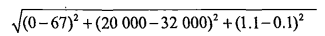
我们很容易发现，上面方程中数字差值最大的属性对计算结果的影响最大，也就是说，每年
获取的飞行常客里程数对于计算结果的影响将远远大于表2-3中其他两个特征—— 玩视频游戏的
和每周消费冰洪淋公升数—— 的影响。而产生这种现象的唯一原因，仅仅是因为飞行常客里程数
远大于其他特征值。但海伦认为这三种特征是同等重要的，因此作为三个等权重的特征之一，飞
行常客里程数并不应该如此严重地影响到计算结果。

在处理这种不同取值范围的特征值时，我们通常采用的方法是将数值归一化，如将取值范围
处理为0到1或者-1到1之间。下面的公式可以将任意取值范围的特征值转化为0到1区间内的值：

其中min 和max乂分别是数据集中的最小特征值和最大特征值。虽然改变数值取值范围增加了
分类器的复杂度，但为了得到准确结果，我们必须这样做。

增加一个
新函数抓autoNorm该函数可以自动将数字特征值转化为0到1的区间。

def autoNorm(dataSet):
    minVals = dataSet.min(0)
    maxVals = dataSet.max(0)
    ranges = maxVals - minVals
    normDataSet = zeros(shape(dataSet))
    m = dataSet.shape[0]
    normDataSet = dataSet - tile(minVals, (m,1))
    normDataSet = normDataSet/tile(ranges, (m,1))   #element wise divide
    return normDataSet, ranges, minVals

normDataSet, ranges, minVals = autoNorm(returnMat)
print(normDataSet)

 测试算法：作为完整程序验证分类器

机器学习算法一个很
重要的工作就是评估算法的正确率，通常我们只提供已有数据的90%作为训练样本来训练分类
器 ，而使用其余的10%数据去测试分类器，检测分类器的正确率。

10%的测试数据应该
是随机选择的，由于海伦提供的数据并没有按照特定目的来排序，所以我们可以随意选择10%数
据而不影响其随机性.

前面我们巳经提到可以使用错误率来检测分类器的性能。对于分类器来说，错误率就是分类
器给出错误结果的次数除以测试数据的总数，完美分类器的错误率为0，而错误率为1.0的分类器
不会给出任何正确的分类结果。代码里我们定义一个计数器变量，每次分类器错误地分类数据，
计数器就加1, 程序执行完成之后计数器的结果除以数据点总数即是错误率。

分类器针对约会网站的测试代码

def datingClassTest():
    hoRatio = 0.50      #hold out 10%
    datingDataMat,datingLabels = file2matrix('F:\machinelearninginaction\Ch02\datingTestSet2.txt')       #load data setfrom file
    normMat, ranges, minVals = autoNorm(datingDataMat)
    m = normMat.shape[0]
    numTestVecs = int(m*hoRatio)
    errorCount = 0.0
    for i in range(numTestVecs):
        classifierResult = classify0(normMat[i,:],normMat[numTestVecs:m,:],datingLabels[numTestVecs:m],3)
        print("the classifier came back with: %d, the real answer is: %d" % (classifierResult, datingLabels[i]))
        if (classifierResult != datingLabels[i]): 
            errorCount += 1.0
    print("the total error rate is: %f" % (errorCount/float(numTestVecs)))
    print(errorCount)
    
datingClassTest()

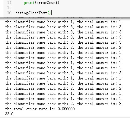
 算法预测错误率大约是：6.6%，算是很不错的了。

使用算法：构建完整可用系统

上面我们已经在数据上对分类器进行了测试，现在终于可以使用这个分类器为海伦来对人们
分类。我们会给海伦一小段程序，通过该程序海伦会在约会网站上找到某个人并输入他的信息。
程序会给出她对对方喜欢程度的预测值。

def classifyPerson():
    resultList = ['not at all','in small doses1','in large doses'] 
    percentTats = float(input("percentage of time spent playing video games?"))
    ffMiles = float(input("freguent flier miles earned per year?"))
    iceCream = float(input('liters of ice cream consumed per year?')) 
    datingDataMat,datingLabels = file2matrix('F:\machinelearninginaction\Ch02\datingTestSet2.txt') 
    normMat, ranges, minVals = autoNorm(datingDataMat) 
    inArr = array([ffMiles, percentTats, iceCream])
    classifierResult = classify0((inArr-minVals)/ranges,normMat,datingLabels,3) 
    print("You will probably like this person：",resultList[classifierResult - 1])
    
classifyPerson()