TensorFlow激活函数+归一化-函数

激活函数的作用如下-引用《TensorFlow实践》：

  这些函数与其他层的输出联合使用可以生成特征图。他们用于对某些运算的结果进行平滑或者微分。其目标是为神经网络引入非线性。曲线能够刻画出输入的复杂的变化。TensorFlow提供了多种激活函数，在CNN中一般使用tf.nn.relu的原因是因为，尽管relu会导致一些信息的损失，但是性能突出。在刚开始设计模型时，都可以采用relu的激活函数。高级用户也可以自己创建自己的激活函数，评价激活函数是否有用的主要因素参看如下几点：

1）该函数是单调的，随着输入的增加增加减小减小，从而利用梯度下降法找到局部极值点成为可能。

2）该函数是可微分的，以保证函数定义域内的任意一点上导数都存在，从而使得梯度下降法能够正常使用来自这类激活函数的输出。

常见的TensorFlow提供的激活函数如下：(详细请参考http://www.tensorfly.cn/tfdoc/api_docs/python/nn.html)

1.tf.nn.relu(features, name=None)

Computes rectified linear: max(features, 0).

• features: A Tensor. Must be one of the following types: float32, float64, int32, int64,uint8, int16, int8.
• name: A name for the operation (optional).

注：

优点在于不受‘梯度消失’的影响，取值范围为[0，+∞]。

缺点在于当使用了较大的学习速率时，易受到饱和的神经元的影响。

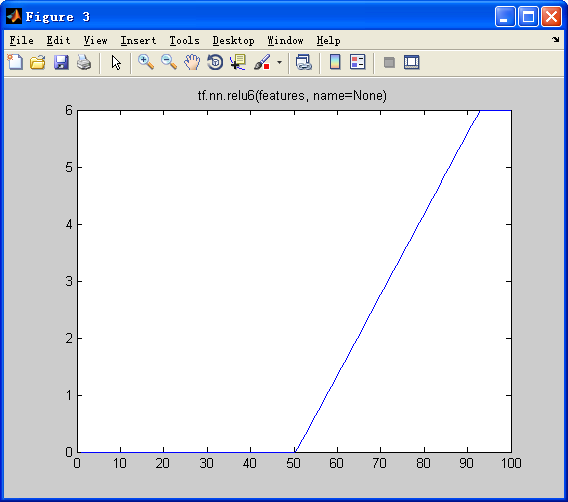
2.tf.nn.relu6(features, name=None)

Computes Rectified Linear 6: min(max(features, 0), 6).

• features: A Tensor with type float, double, int32, int64, uint8, int16, or int8.
• name: A name for the operation (optional).

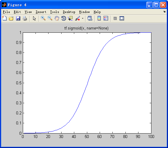
3.tf.sigmoid(x, name=None)

Computes sigmoid of x element-wise.

Specifically, y = 1 / (1 + exp(-x)).

• x: A Tensor with type float, double, int32, complex64, int64, or qint32.
• name: A name for the operation (optional).

注：

优点在于sigmoid函数在样本训练的神经网络中可以将输出保持在[0.0,1.0]内部的能力非常有用。

缺点在于当输出接近饱和或剧烈变化时，对输出范围的这种缩减往往会带来一些不利影响。

4.tf.nn.softplus(features, name=None)

Computes softplus: log(exp(features) + 1).

• features: A Tensor. Must be one of the following types: float32, float64, int32, int64,uint8, int16, int8.
• name: A name for the operation (optional).

5.tf.tanh(x, name=None)

Computes hyperbolic tangent of x element-wise.

• x: A Tensor with type float, double, int32, complex64, int64, or qint32.
• name: A name for the operation (optional).

注：

优点在于双曲正切函数和sigmoid函数比较相似，tanh拥有sigmoid的优点，用时tanh具有输出负值的能力，tanh的值域为[-1.0,1.0].

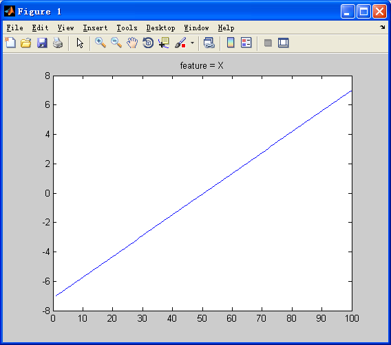
MATLAB代码来体现函数的类型

clear all
close all
clc
% ACTVE FUNCTION %
X = linspace(-5,5,100);
plot(X)
title('feature = X')
% tf.nn.relu(features, name=None):max(features, 0) %
Y_relu = max(X,0);
figure,plot(Y_relu)
title('tf.nn.relu(features, name=None)')
% tf.nn.relu6(features, name=None):min(max(features, 0), 6) %
Y_relu6 = min(max(X,0),6);
figure,plot(Y_relu6)
title('tf.nn.relu6(features, name=None)')
% tf.sigmoid(x, name=None):y = 1 / (1 + exp(-x))%
Y_sigmoid = 1./(1+exp(-1.*X));
figure,plot(Y_sigmoid)
title('tf.sigmoid(x, name=None)')
% tf.nn.softplus(features, name=None):log(exp(features) + 1) %
Y_softplus = log(exp(X) + 1);
figure,plot(Y_softplus)
title('tf.nn.softplus(features, name=None)')
% tf.tanh(x, name=None):tanh(features) %
Y_tanh = tanh(X);
figure,plot(Y_tanh)
title('tf.tanh(x, name=None)')

                             X=feature                                 tf.nn.relu(features, name=None)    

       tf.nn.relu6(features, name=None)                         tf.sigmoid(x, name=None)

           tf.nn.softplus(features, name=None)                        tf.tanh(x, name=None)

归一化函数的重要作用-引用《TensorFlow实践》：

  归一化层并非CNN所独有。在使用tf.nn.relu时，考虑输出的归一化是有价值的（详细参看http://papers.nips.cc/paper/4824-imagenet-classification-with-deep-convolutional-neural-networks.pdf）。由于relu是无界函数，利用某些形式的归一化来识别哪些高频特征通常是十分有用的。local response normalization最早是由Krizhevsky和Hinton在关于ImageNet的论文里面使用的一种数据标准化方法，即使现在，也依然会有不少CNN网络会使用到这种正则手段。

tf.nn.local_response_normalization(input, depth_radius=None, bias=None, alpha=None, beta=None, name=None)

Local Response Normalization.

The 4-D input tensor is treated as a 3-D array of 1-D vectors (along the last dimension), and each vector is normalized independently. Within a given vector, each component is divided by the weighted, squared sum of inputs within depth_radius. In detail,

sqr_sum[a, b, c, d] =
    sum(input[a, b, c, d - depth_radius : d + depth_radius + 1] ** 2)
output = input / (bias + alpha * sqr_sum ** beta)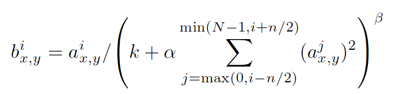

• 第一个参数input：这个输入就是feature map了，既然是feature map，那么它就具有[batch, height, width, channels]这样的shape
• 第二个参数depth_radius：这个值需要自己指定，就是上述公式中的n/2
• 第三个参数bias：上述公式中的k
• 第四个参数alpha：上述公式中的α
• 第五个参数beta：上述公式中的β
• 第六个参数name：上述操作的名称
• 返回值是新的feature map，它应该具有和原feature map相同的shape

以上是这种归一手段的公式，其中a的上标指该层的第几个feature map，a的下标x，y表示feature map的像素位置，N指feature map的总数量，公式里的其它参数都是超参，需要自己指定的。

这种方法是受到神经科学的启发，激活的神经元会抑制其邻近神经元的活动（侧抑制现象），至于为什么使用这种正则手段，以及它为什么有效，查阅了很多文献似乎也没有详细的解释，可

能是由于后来提出的batch normalization手段太过火热，渐渐的就把local response normalization掩盖了吧。

import tensorflow as tf  
  
a = tf.constant([  
    [[1.0, 2.0, 3.0, 4.0],  
     [5.0, 6.0, 7.0, 8.0],  
     [8.0, 7.0, 6.0, 5.0],  
     [4.0, 3.0, 2.0, 1.0]],  
    [[4.0, 3.0, 2.0, 1.0],  
     [8.0, 7.0, 6.0, 5.0],  
     [1.0, 2.0, 3.0, 4.0],  
     [5.0, 6.0, 7.0, 8.0]]  
])  
#reshape a,get the feature map [batch:1 height:2 2 channels:8]  
a = tf.reshape(a, [1, 2, 2, 8])  
  
normal_a=tf.nn.local_response_normalization(a,2,0,1,1)  
with tf.Session() as sess:  
    print("feature map:")  
    image = sess.run(a)  
    print (image)  
    print("normalized feature map:")  
    normal = sess.run(normal_a)  
    print (normal)  

运行结果：

解释：

这里我取了n/2=2，k=0，α=1，β=1。公式中的N就是输入张量的通道总数：由a = tf.reshape(a, [1, 2, 2, 8]) 得到 N=8，变量i代表的是不同的通道，从0开始到7.

举个例子，比如对于一通道的第一个像素“1”来说，我们把参数代人公式就是1/(1^2+2^2+3^2)=0.07142857，对于四通道的第一个像素“4”来说，公式就是4/（2^2+3^2+4^2+5^2+6^2）=0.04444445，以此类推。转载：http://blog.csdn.net/mao_xiao_feng/article/details/53488271