机器学习笔记（四）Logistic回归模型实现

 一、Logistic回归实现

（一）特征值较少的情况

1. 实验数据

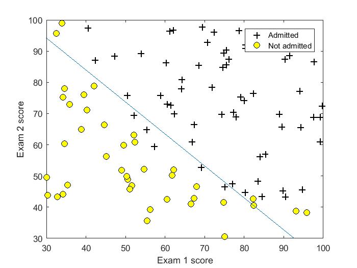
吴恩达《机器学习》第二课时作业提供数据1。判断一个学生能否被一个大学录取，给出的数据集为学生两门课的成绩和是否被录取，通过这些数据来预测一个学生能否被录取。

2. 分类结果评估

横纵轴（特征）为学生两门课成绩，可以在图中清晰地画出决策边界。

3. 代码实现

 首先自己实现了梯度下降方法并测试

 gradientDesent.m

%Logistic gradientDesent
function [Theta] = gradientDescentLog(X, y, Theta, alpha, counter)
[m,n] = size(X); % m样本数量 n特征数
H = zeros(m,1);
for iter = 1:counter
    H =  1./(1 + exp(X * Theta));
    Delta = (1/m) * X'*(H-y)  
    Theta = Theta + alpha * Delta;
    Jtheta = (-1/m)*(y'*log(H)+(1-y)'*log(1-H))
end

接下来用课程中讲的高级优化方法，并实现costFunction函数。

%% Machine Learning Online Class - Exercise 2: Logistic Regression % 
%% Initialization 
clear ; close all; clc 
%% Load Data 
%  The first two columns contains the exam scores and the third column 
%  contains the label. 
data = load('ex2data1.txt'); 
X = data(:, [1, 2]); 
y = data(:, 3); 
%% ==================== Part 1: Plotting ==================== 
%We start the exercise by first plotting the data to understand the 
%  the problem we are working with. 
fprintf(['Plotting data with + indicating (y = 1) examples and o ' ...
         'indicating (y = 0) examples.
']); 
plotData(X, y); 
xlabel('Exam 1 score') 
ylabel('Exam 2 score') 
legend('Admitted', 'Not admitted') 
hold off; 
fprintf('
Program paused. Press enter to continue.
'); 
pause; 
%% ============ Part 2: Compute Cost and Gradient ============ 
[m, n] = size(X); 
% Add intercept term to x and X_test 
X = [ones(m, 1) X]; 
% Initialize fitting parameters 
initial_theta = zeros(n + 1, 1); 
% Compute and display initial cost and gradient 
[cost, grad] = costFunction(initial_theta, X, y); 
fprintf('Cost at initial theta (zeros): %f
', cost); 
fprintf('Expected cost (approx): 0.693
'); 
fprintf('Gradient at initial theta (zeros): 
'); 
fprintf(' %f 
', grad); 
fprintf('Expected gradients (approx):
 -0.1000
 -12.0092
 -11.2628
');
 % Compute and display cost and gradient with non-zero theta 
test_theta = [-24; 0.2; 0.2]; 
[cost, grad] = costFunction(test_theta, X, y); 
fprintf('
Cost at test theta: %f
', cost); 
fprintf('Expected cost (approx): 0.218
'); 
fprintf('Gradient at test theta: 
'); 
fprintf(' %f 
', grad); 
fprintf('Expected gradients (approx):
 0.043
 2.566
 2.647
'); 
fprintf('
Program paused. Press enter to continue.
'); 
pause; 
%% ============= Part 3: Optimizing using fminunc  ============= 
%  Set options for fminunc 
options = optimset('GradObj', 'on', 'MaxIter', 40); 
%  Run fminunc to obtain the optimal theta 
%  This function will return theta and the cost 
[theta, cost] = ... 
    fminunc(@(t)(costFunction(t, X, y)), initial_theta, options);
% Print theta to screen 
fprintf('Cost at theta found by fminunc: %f
', cost); 
fprintf('Expected cost (approx): 0.203
'); 
fprintf('theta: 
'); 
fprintf(' %f 
', theta); 
fprintf('Expected theta (approx):
');
fprintf(' -25.161
 0.206
 0.201
'); 
% Plot Boundary 
plotDecisionBoundary(theta, X, y); 
% Put some labels hold on; 
% Labels and Legend 
xlabel('Exam 1 score') 
ylabel('Exam 2 score') 
% Specified in plot order 
legend('Admitted', 'Not admitted') 
hold off; 
fprintf('
Program paused. Press enter to continue.
'); 
pause; 
%% ============== Part 4: Predict and Accuracies ============== 
prob = sigmoid([1 45 85] * theta); 
fprintf(['For a student with scores 45 and 85, we predict an admission ' ...
         'probability of %f
'], prob);
fprintf('Expected value: 0.775 +/- 0.002

'); 
% Compute accuracy on our training set 
p = predict(theta, X); 
fprintf('Train Accuracy: %f
', mean(double(p == y)) * 100); 
fprintf('Expected accuracy (approx): 89.0
'); 
fprintf('
');

 predict.m

function p = predict(theta, X) 
%PREDICT Predict whether the label is 0 or 1 using learned logistic 
m = size(X, 1); 
% Number of training examples 
p = sigmoid(X * theta)>=0.5;
end

 sigmoid.m

function g = sigmoid(z) 
%SIGMOID Compute sigmoid function 
g = zeros(size(z)); 
g = 1./(1 + exp(-z)); 
end

 costFunction.m

function [J, grad] = costFunction(theta, X, y) 
%COSTFUNCTION Compute cost and gradient for logistic regression 
m = length(y); 
% number of training examples 
J = 0; 
grad = zeros(size(theta)); 
J = 1/m*(-y'*log(sigmoid(X*theta)) - (1-y)'*(log(1-sigmoid(X*theta)))); 
grad = 1/m * X'*(sigmoid(X*theta) - y); 
end 

 plotData.m

function plotData(X, y)
pos = find(y == 1); 
neg = find(y == 0);
plot(X(pos, 1), X(pos, 2), 'k+','LineWidth', 1, ...
'MarkerSize', 7);
hold on；
plot(X(neg, 1), X(neg, 2), 'ko', 'MarkerFaceColor', 'y', ...
'MarkerSize', 7);

 plotDecisionBoundary.m（course provide）

function plotDecisionBoundary(theta, X, y)
%函数plotDate
plotData(X(:,2:3), y);
hold on
if size(X, 2) <= 3
    % Only need 2 points to define a line, so choose two endpoints
    plot_x = [min(X(:,2))-2,  max(X(:,2))+2];
    % Calculate the decision boundary line
    plot_y = (-1./theta(3)).*(theta(2).*plot_x + theta(1));
    % Plot, and adjust axes for better viewing
    plot(plot_x, plot_y)
        % Legend, specific for the exercise
    legend('Admitted', 'Not admitted', 'Decision Boundary')
    axis([30, 100, 30, 100])
else
    % Here is the grid range
    u = linspace(-1, 1.5, 50);
    v = linspace(-1, 1.5, 50);
    z = zeros(length(u), length(v));
    % Evaluate z = theta*x over the grid
    for i = 1:length(u)
        for j = 1:length(v)
            z(i,j) = mapFeature(u(i), v(j))*theta;
        end
    end
    z = z'; % important to transpose z before calling contour
    % Plot z = 0
    % Notice you need to specify the range [0, 0]
    contour(u, v, z, [0, 0], 'LineWidth', 2) %画等值线
end
hold off
end

 输出结果：

For a student with scores 45 and 85, we predict an admission probability of 0.771019
Expected value: 0.775 +/- 0.002

Train Accuracy: 89.000000
Expected accuracy (approx): 89.0

（二）特征值较多的情况

1. 实验数据

http://archive.ics.uci.edu/ml/index.php wine数据集，其特征取值是连续的。

2. 分类结果评估

考虑一个二分问题，即将实例分成正类（positive）或负类（negative）。对一个二分问题来说，会出现四种情况：

实例是正类并且也被预测成正类，即为真正类（TP：True positive）

实例是负类被预测成正类，称之为假正类（FP：False positive）

实例是负类被预测成负类，称之为真负类（TN：True negative）

实例是正类被预测成负类则为假负类（FN：false negative）。

评价标准：

精确率：precision = TP / (TP + FP)模型判为正的所有样本中有多少是真正的正样本。

召回率：recall = TP / (TP + FN)

准确率：accuracy = (TP + TN) / (TP + FP + TN + FN)反映了分类器统对整个样本的判定能力——能将正的判定为正，负的判定为负

如何在precision和Recall中权衡？F1 Score = P*R/2(P+R)，其中P和R分别为 precision 和 recall，在precision与recall都要求高的情况下，可以用F1 Score来衡量。

为什么会有这么多指标呢？这是因为模式分类和机器学习的需要。判断一个分类器对所用样本的分类能力或者在不同的应用场合时，需要有不同的指标。

 3. 代码实现

%Logistic回归梯度下降法
%logistic梯度下降法
[Data] = xlsread('wine.xlsx',1,'B1:N130');
[y] = xlsread('wine.xlsx',1,'A1:A130');
[m,n] = size(Data); % m样本数量 n特征数
Data = featureScaling(Data);
for i = 1:m
    if y(i)==2
        y(i) = 0;
    end
end
x0 = ones(m,1);

X = ([x0,Data])';
Theta = zeros(n+1,1);
alpha = 0.1;
counter = 4000;
H = gradientDescentLog(X, y, Theta, alpha, counter);
TP = 0; TN = 0; FP = 0; FN = 0;
for i = 1:m
    if H(i)<0.5 %判断为negative
        if y(i)==0
            TN = TN+1;
        else
            FN = FN+1;
        end
   else  %判断为positive
        if y(i)==1
            TP = TP+1;
        else
            FP = FP+1;
        end
    end
end
precision = TP / (TP + FP)
recall = TP / (TP + FN)
accuracy = (TP + TN) / (TP + FP + TN + FN)

%Logistic gradientDesent
function [H] = gradientDescentLog(X, y, Theta, alpha, counter)
[n,m] = size(X); % m样本数量 n特征数
H = zeros(m,1);
for iter = 1:counter
    for i = 1:m
        H(i) = 1/(1+exp(-Theta'*X(:,i))); %Logistic回归模型
    end
    Delta = 1/m * X * (H-y);
    Theta = Theta - alpha * Delta;
    Jtheta = -1/m*(y'*log(H)+(1-y)'*log(1-H))
end

输出结果：

Jtheta = 0.3497
precision = 0.8983
recall = 0.8983
accuracy = 0.9077

此时alpha = 0.1; counter = 4000;可见此时很可能已经出现过拟合现象，在下一篇笔记中我们针对这种过拟合现象进行讨论。