机器学习：SVM（scikit-learn 中的 SVM：LinearSVC）

一、基础理解

• Hard Margin SVM 和 Soft Margin SVM 都是解决线性分类问题，无论是线性可分的问题，还是线性不可分的问题；

• 和 kNN 算法一样，使用 SVM 算法前，要对数据做标准化处理；
• 原因：SVM 算法中设计到计算 Margin 距离，如果数据点在不同的维度上的量纲不同，会使得距离的计算有问题；
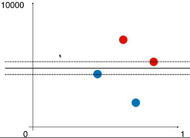
• 例如：样本的两种特征，如果相差太大，使用 SVM 经过计算得到的决策边界几乎为一条水平的直线——因为两种特征的数据量纲相差太大，水平方向的距离可以忽略，因此，得到的最大的 Margin 就是两条虚线的垂直距离；
• 
• 只有不同特征的数据的量纲一样时，得到的决策边界才没有问题；

二、例

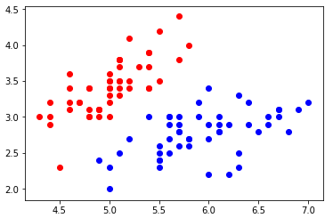
　1）导入并绘制数据集

• import numpy as np
  import matplotlib.pyplot as plt
  from sklearn import datasets
  
  iris = datasets.load_iris()
  X = iris.data
  y = iris.target
  X = X[y<2, :2]
  y = y[y<2]
  
  plt.scatter(X[y==0, 0], X[y==0, 1], color='red')
  plt.scatter(X[y==1, 0], X[y==1, 1], color='blue')
  plt.show()

  

　2）LinearSVC（线性 SVM 算法）

• LinearSVC：该算法使用了支撑向量机的思想；
• 数据标准化

  from sklearn.preprocessing import StandardScaler
  
  standardScaler = StandardScaler()
  standardScaler.fit(X)
  X_standard = standardScaler.transform(X)

• 调用 LinearSVC

  from sklearn.svm import LinearSVC
  
  svc = LinearSVC(C=10**9)
  svc.fit(X_standard, y)

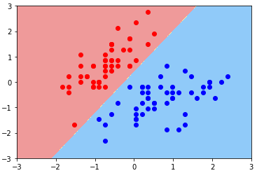
• 导入绘制决策边界的函数，并绘制模型决策边界：Hard Margin SVM 思想

  def plot_decision_boundary(model, axis):
      
      x0, x1 = np.meshgrid(
          np.linspace(axis[0], axis[1], int((axis[1]-axis[0])*100)).reshape(-1,1),
          np.linspace(axis[2], axis[3], int((axis[3]-axis[2])*100)).reshape(-1,1)
      )
      X_new = np.c_[x0.ravel(), x1.ravel()]
      
      y_predict = model.predict(X_new)
      zz = y_predict.reshape(x0.shape)
      
      from matplotlib.colors import ListedColormap
      custom_cmap = ListedColormap(['#EF9A9A','#FFF59D','#90CAF9'])
      
      plt.contourf(x0, x1, zz, linewidth=5, cmap=custom_cmap)
  
  plot_decision_boundary(svc, axis=[-3, 3, -3, 3])
  plt.scatter(X_standard[y==0, 0], X_standard[y==0, 1], color='red')
  plt.scatter(X_standard[y==1, 0], X_standard[y==1, 1], color='blue')
  plt.show()

  

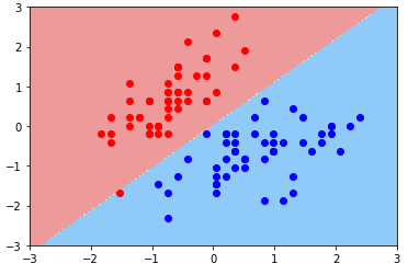
• 绘制决策边界：Soft Margin SVM 思想

  svc2 = LinearSVC(C=0.01)
  svc2.fit(X_standard, y)
  
  plot_decision_boundary(svc2, axis=[-3, 3, -3, 3])
  plt.scatter(X_standard[y==0, 0], X_standard[y==0, 1], color='red')
  plt.scatter(X_standard[y==1, 0], X_standard[y==1, 1], color='blue')
  plt.show()

  

　3）绘制支撑向量所在的直线

• svc.coef_：算法模型的系数，有两个值，因为样本有两种特征，每个特征对应一个系数；
• 系数：特征与样本分类结果的关系系数；
• svc.intercept_：模型的截距，一维向量，只有一个数，因为只有一条直线；

• 系数：w = svc.coef_
• 截距：b = svc.intercept_
• 决策边界直线方程：w[0] * x0 + w[1] * x1 + b = 0
• 支撑向量直线方程：w[0] * x0 + w[1] * x1 + b = ±1
• 变形：

1. 决策边界：x1 = -w[0]/w[1] * x0 - b/w[1]
2. 支撑向量：x1 = -w[0]/w[1] * x0 - b/w[1] ± 1/w[1]

• 修改绘图函数

  # 绘制：决策边界、支撑向量所在的直线
  def plot_svc_decision_boundary(model, axis):
      
      x0, x1 = np.meshgrid(
          np.linspace(axis[0], axis[1], int((axis[1]-axis[0])*100)).reshape(-1,1),
          np.linspace(axis[2], axis[3], int((axis[3]-axis[2])*100)).reshape(-1,1)
      )
      X_new = np.c_[x0.ravel(), x1.ravel()]
      
      y_predict = model.predict(X_new)
      zz = y_predict.reshape(x0.shape)
      
      from matplotlib.colors import ListedColormap
      custom_cmap = ListedColormap(['#EF9A9A','#FFF59D','#90CAF9'])
      
      plt.contourf(x0, x1, zz, linewidth=5, cmap=custom_cmap)
      
      w = model.coef_[0]
      b = model.intercept_[0]
      
      plot_x = np.linspace(axis[0], axis[1], 200)
      up_y = -w[0]/w[1] * plot_x - b/w[1] + 1/w[1]
      down_y = -w[0]/w[1] * plot_x - b/w[1] - 1/w[1]
      
      # 将 plot_x 与 up_y、down_y 的关系以折线图的形式表示出来
      # 此处有一个问题：up_y和down_y的结果可能超过了 axis 中 y 坐标的范围，需要添加一个过滤条件：
      # up_index：布尔向量，元素 True 表示，up_y 中的满足 axis 中的 y 的范围的值在 up_y 中的引索；
      # down_index：布尔向量，同理 up_index;
      up_index = (up_y >= axis[2]) & (up_y <= axis[3])
      down_index = (down_y >= axis[2]) & (down_y <= axis[3])
      plt.plot(plot_x[up_index], up_y[up_index], color='black')
      plt.plot(plot_x[down_index], down_y[down_index], color='black')

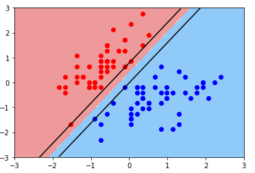
• 绘图：Hard Margin SVM

  plot_svc_decision_boundary(svc, axis=[-3, 3, -3, 3])
  plt.scatter(X_standard[y==0, 0], X_standard[y==0, 1], color='red')
  plt.scatter(X_standard[y==1, 0], X_standard[y==1, 1], color='blue')
  plt.show()

  

• 绘图：Soft Margin SVM

  plot_svc_decision_boundary(svc2, axis=[-3, 3, -3, 3])
  plt.scatter(X_standard[y==0, 0], X_standard[y==0, 1], color='red')
  plt.scatter(X_standard[y==1, 0], X_standard[y==1, 1], color='blue')
  plt.show()

  

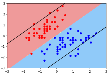
• 现象：Margin 非常大，中间容错了很多样本点；
• 原因：C 超参数过小，模型容错空间过大；
• 方案：调参；