import scvelo as scv
adata = scv.read("E:/data_exercise/day1_27/scV/data/Pancreas/adata_dynamics.h5ad", cache=True)
adata
AnnData object with n_obs × n_vars = 3696 × 2000
    obs: 'clusters_coarse', 'clusters', 'S_score', 'G2M_score', 'initial_size_spliced', 'initial_size_unspliced', 'initial_size', 'n_counts'
    var: 'highly_variable_genes', 'gene_count_corr', 'means', 'dispersions', 'dispersions_norm', 'highly_variable', 'fit_r2', 'fit_alpha', 'fit_beta', 'fit_gamma', 'fit_t_', 'fit_scaling', 'fit_std_u', 'fit_std_s', 'fit_likelihood', 'fit_u0', 'fit_s0', 'fit_pval_steady', 'fit_steady_u', 'fit_steady_s', 'fit_variance', 'fit_alignment_scaling'
    uns: 'clusters_coarse_colors', 'clusters_colors', 'day_colors', 'neighbors', 'pca', 'recover_dynamics'
    obsm: 'X_pca', 'X_umap'
    varm: 'loss'
    layers: 'Ms', 'Mu', 'fit_t', 'fit_tau', 'fit_tau_', 'spliced', 'unspliced'
    obsp: 'connectivities', 'distances'
# 计算速度矢量
scv.tl.velocity(adata, mode='dynamical')
scv.tl.velocity_graph(adata)
computing velocities
    finished (0:00:06) --> added
    'velocity', velocity vectors for each individual cell (adata.layers)
computing velocity graph
    finished (0:00:11) --> added
    'velocity_graph', sparse matrix with cosine correlations (adata.uns)
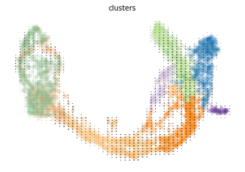
#汇出嵌入模型
scv.pl.velocity_embedding_grid(adata, basis='umap')
computing velocity embedding
    finished (0:00:01) --> added
    'velocity_umap', embedded velocity vectors (adata.obsm)
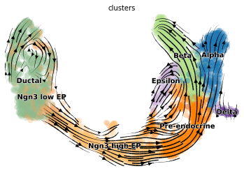
#汇出嵌入模型
scv.pl.velocity_embedding_stream(adata, basis='umap')
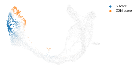
#计算cell cycle score并可视化
scv.tl.score_genes_cell_cycle(adata)

scv.pl.scatter(adata, color_gradients=['S_score', 'G2M_score'], basis="umap", smooth=True, perc=[5, 95])
calculating cell cycle phase
-->     'S_score' and 'G2M_score', scores of cell cycle phases (adata.obs)
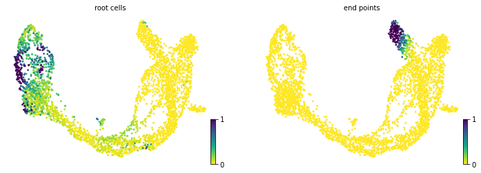
#3.5 计算细胞状态并可视化

scv.tl.terminal_states(adata)

scv.pl.scatter(adata, color=[ 'root_cells', 'end_points'], basis='umap')
#'root_cells', root cells of Markov diffusion process (adata.obs)
#'end_points', end points of Markov diffusion process (adata.obs)
computing terminal states
WARNING: Uncertain or fuzzy root cell identification. Please verify.
    identified 2 regions of root cells and 1 region of end points .
    finished (0:00:00) --> added
    'root_cells', root cells of Markov diffusion process (adata.obs)
    'end_points', end points of Markov diffusion process (adata.obs)
adata
AnnData object with n_obs × n_vars = 3696 × 2000
    obs: 'clusters_coarse', 'clusters', 'S_score', 'G2M_score', 'initial_size_spliced', 'initial_size_unspliced', 'initial_size', 'n_counts', 'velocity_self_transition', 'phase', 'clusters_gradients', 'root_cells', 'end_points'
    var: 'highly_variable_genes', 'gene_count_corr', 'means', 'dispersions', 'dispersions_norm', 'highly_variable', 'fit_r2', 'fit_alpha', 'fit_beta', 'fit_gamma', 'fit_t_', 'fit_scaling', 'fit_std_u', 'fit_std_s', 'fit_likelihood', 'fit_u0', 'fit_s0', 'fit_pval_steady', 'fit_steady_u', 'fit_steady_s', 'fit_variance', 'fit_alignment_scaling', 'velocity_genes'
    uns: 'clusters_coarse_colors', 'clusters_colors', 'day_colors', 'neighbors', 'pca', 'recover_dynamics', 'velocity_params', 'velocity_graph', 'velocity_graph_neg', 'clusters_gradients_colors'
    obsm: 'X_pca', 'X_umap', 'velocity_umap'
    varm: 'loss'
    layers: 'Ms', 'Mu', 'fit_t', 'fit_tau', 'fit_tau_', 'spliced', 'unspliced', 'velocity', 'velocity_u'
    obsp: 'connectivities', 'distances'
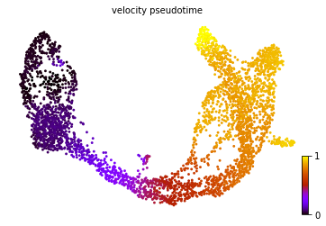
#计算pseudotime,可视化,与导出

scv.tl.velocity_pseudotime(adata)

scv.pl.scatter(adata=adata, color='velocity_pseudotime', cmap='gnuplot', basis="umap")

adata.obs["velocity_pseudotime"].to_csv('velocyto_pseudotime.csv')
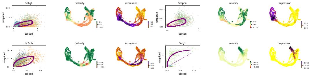
#查看特定基因的velocity

var_names = ['Snhg6', 'Sbspon', 'Eif2s3y', 'Sntg1'] #adata.var 下的index就是基因名

scv.pl.velocity(adata, var_names=var_names, colorbar=True, ncols=2)
adata
AnnData object with n_obs × n_vars = 3696 × 2000
    obs: 'clusters_coarse', 'clusters', 'S_score', 'G2M_score', 'initial_size_spliced', 'initial_size_unspliced', 'initial_size', 'n_counts', 'velocity_self_transition', 'phase', 'clusters_gradients', 'root_cells', 'end_points', 'velocity_pseudotime'
    var: 'highly_variable_genes', 'gene_count_corr', 'means', 'dispersions', 'dispersions_norm', 'highly_variable', 'fit_r2', 'fit_alpha', 'fit_beta', 'fit_gamma', 'fit_t_', 'fit_scaling', 'fit_std_u', 'fit_std_s', 'fit_likelihood', 'fit_u0', 'fit_s0', 'fit_pval_steady', 'fit_steady_u', 'fit_steady_s', 'fit_variance', 'fit_alignment_scaling', 'velocity_genes'
    uns: 'clusters_coarse_colors', 'clusters_colors', 'day_colors', 'neighbors', 'pca', 'recover_dynamics', 'velocity_params', 'velocity_graph', 'velocity_graph_neg', 'clusters_gradients_colors'
    obsm: 'X_pca', 'X_umap', 'velocity_umap'
    varm: 'loss'
    layers: 'Ms', 'Mu', 'fit_t', 'fit_tau', 'fit_tau_', 'spliced', 'unspliced', 'velocity', 'velocity_u'
    obsp: 'connectivities', 'distances'
df = adata.var
df
| highly_variable_genes | gene_count_corr | means | dispersions | dispersions_norm | highly_variable | fit_r2 | fit_alpha | fit_beta | fit_gamma | ... | fit_std_s | fit_likelihood | fit_u0 | fit_s0 | fit_pval_steady | fit_steady_u | fit_steady_s | fit_variance | fit_alignment_scaling | velocity_genes | |
|---|---|---|---|---|---|---|---|---|---|---|---|---|---|---|---|---|---|---|---|---|---|
| index | |||||||||||||||||||||
| Sntg1 | True | NaN | 0.005065 | 0.131135 | 0.214469 | True | 0.401981 | 0.015726 | 0.005592 | 0.088792 | ... | 0.030838 | 0.406523 | 0.0 | 0.0 | 0.159472 | 2.470675 | 0.094304 | 0.149138 | 5.355590 | False |
| Snhg6 | False | NaN | 0.375835 | 0.158585 | 0.040765 | True | 0.125072 | 0.389126 | 2.981982 | 0.260322 | ... | 0.245248 | 0.243441 | 0.0 | 0.0 | 0.403409 | 0.106128 | 0.596630 | 0.762252 | 2.037296 | True |
| Ncoa2 | False | NaN | 0.106945 | 0.145879 | 0.298358 | True | -2.313923 | NaN | NaN | NaN | ... | NaN | NaN | NaN | NaN | NaN | NaN | NaN | NaN | NaN | False |
| Sbspon | True | NaN | 0.143032 | 0.277016 | 1.044508 | True | 0.624803 | 0.464865 | 2.437113 | 0.379645 | ... | 0.178859 | 0.252135 | 0.0 | 0.0 | 0.182088 | 0.164805 | 0.430623 | 0.674312 | 1.193015 | True |
| Ube2w | False | NaN | 0.018522 | 0.109459 | 0.091136 | True | -5.324582 | NaN | NaN | NaN | ... | NaN | NaN | NaN | NaN | NaN | NaN | NaN | NaN | NaN | False |
| ... | ... | ... | ... | ... | ... | ... | ... | ... | ... | ... | ... | ... | ... | ... | ... | ... | ... | ... | ... | ... | ... |
| Tmem27 | True | NaN | 1.297619 | 2.475960 | 3.254982 | True | 0.527855 | 3.954723 | 21.314334 | 0.253763 | ... | 5.014219 | 0.292956 | 0.0 | 0.0 | 0.496411 | 0.168456 | 12.425889 | 0.389388 | 3.163113 | False |
| Uty | False | NaN | 0.018673 | 0.182256 | 0.505338 | True | -0.555835 | NaN | NaN | NaN | ... | NaN | NaN | NaN | NaN | NaN | NaN | NaN | NaN | NaN | False |
| Ddx3y | True | NaN | 0.165256 | 0.350978 | 1.465338 | True | -2.538731 | NaN | NaN | NaN | ... | NaN | NaN | NaN | NaN | NaN | NaN | NaN | NaN | NaN | False |
| Eif2s3y | True | NaN | 0.182643 | 0.318686 | 1.281603 | True | 0.352190 | 0.193458 | 0.746410 | 0.295085 | ... | 0.158051 | 0.262140 | 0.0 | 0.0 | 0.390710 | 0.219716 | 0.424033 | 0.748614 | 2.312621 | True |
| Erdr1 | True | NaN | 0.344720 | 0.215833 | 0.288351 | True | -0.193263 | NaN | NaN | NaN | ... | NaN | NaN | NaN | NaN | NaN | NaN | NaN | NaN | NaN | False |
2000 rows × 23 columns
df.to_csv("adata.var.csv",index=True, header=True )
# 数据框筛选那些基因
df = df[(df['fit_likelihood'] > .1) & df['velocity_genes'] == True]

kwargs = dict(xscale='log', fontsize=16)
df
| highly_variable_genes | gene_count_corr | means | dispersions | dispersions_norm | highly_variable | fit_r2 | fit_alpha | fit_beta | fit_gamma | ... | fit_std_s | fit_likelihood | fit_u0 | fit_s0 | fit_pval_steady | fit_steady_u | fit_steady_s | fit_variance | fit_alignment_scaling | velocity_genes | |
|---|---|---|---|---|---|---|---|---|---|---|---|---|---|---|---|---|---|---|---|---|---|
| index | |||||||||||||||||||||
| Snhg6 | False | NaN | 0.375835 | 0.158585 | 0.040765 | True | 0.125072 | 0.389126 | 2.981982 | 0.260322 | ... | 0.245248 | 0.243441 | 0.0 | 0.0 | 0.403409 | 0.106128 | 0.596630 | 0.762252 | 2.037296 | True |
| Sbspon | True | NaN | 0.143032 | 0.277016 | 1.044508 | True | 0.624803 | 0.464865 | 2.437113 | 0.379645 | ... | 0.178859 | 0.252135 | 0.0 | 0.0 | 0.182088 | 0.164805 | 0.430623 | 0.674312 | 1.193015 | True |
| Fam135a | True | NaN | 0.257955 | 0.171546 | 0.096820 | True | 0.384662 | 0.172335 | 0.118088 | 0.204538 | ... | 0.149868 | 0.283343 | 0.0 | 0.0 | 0.387921 | 1.345830 | 0.393197 | 0.671096 | 3.390194 | True |
| Tbc1d8 | True | NaN | 0.070612 | 0.123167 | 0.169130 | True | 0.613194 | 0.083656 | 0.118139 | 0.227401 | ... | 0.081595 | 0.246594 | 0.0 | 0.0 | 0.392402 | 0.659434 | 0.240100 | 0.829478 | 2.914215 | True |
| Fhl2 | True | NaN | 0.232482 | 0.818012 | 2.892669 | True | 0.325223 | 0.224027 | 0.330934 | 0.121456 | ... | 0.317963 | 0.262849 | 0.0 | 0.0 | 0.476793 | 0.539878 | 1.073687 | 0.695997 | 4.785407 | True |
| ... | ... | ... | ... | ... | ... | ... | ... | ... | ... | ... | ... | ... | ... | ... | ... | ... | ... | ... | ... | ... | ... |
| Map3k15 | True | NaN | 0.180941 | 0.427601 | 1.901315 | True | 0.437069 | 0.252467 | 0.348783 | 0.275921 | ... | 0.225956 | 0.289070 | 0.0 | 0.0 | 0.434454 | 0.611380 | 0.560048 | 0.510572 | 2.208756 | True |
| Rai2 | True | NaN | 0.231965 | 0.651755 | 2.173640 | True | 0.769033 | 0.792172 | 2.885604 | 0.647345 | ... | 0.276047 | 0.271263 | 0.0 | 0.0 | 0.311969 | 0.243741 | 0.716996 | 0.707595 | 1.063908 | True |
| Rbbp7 | False | NaN | 1.017536 | 0.422314 | 0.153713 | True | 0.344213 | 1.446806 | 5.332362 | 0.326539 | ... | 0.796754 | 0.281498 | 0.0 | 0.0 | 0.477365 | 0.208398 | 2.985787 | 0.704522 | 2.100311 | True |
| Ap1s2 | True | NaN | 0.127856 | 0.319473 | 1.286081 | True | 0.716659 | 0.202643 | 0.596662 | 0.392769 | ... | 0.140455 | 0.286893 | 0.0 | 0.0 | 0.140955 | 0.315635 | 0.366964 | 0.671211 | 1.775751 | True |
| Eif2s3y | True | NaN | 0.182643 | 0.318686 | 1.281603 | True | 0.352190 | 0.193458 | 0.746410 | 0.295085 | ... | 0.158051 | 0.262140 | 0.0 | 0.0 | 0.390710 | 0.219716 | 0.424033 | 0.748614 | 2.312621 | True |
1006 rows × 23 columns
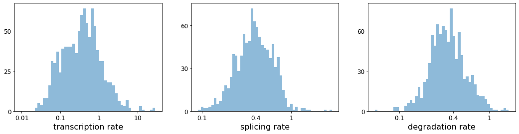
#RNA转录,剪接和降解的速率。
with scv.GridSpec(ncols=3) as pl:
    pl.hist(df['fit_alpha'], xlabel='transcription rate', **kwargs)
    pl.hist(df['fit_beta'] * df['fit_scaling'], xlabel='splicing rate', xticks=[.1, .4, 1], **kwargs)
    pl.hist(df['fit_gamma'], xlabel='degradation rate', xticks=[.1, .4, 1], **kwargs)
adata
AnnData object with n_obs × n_vars = 3696 × 2000
    obs: 'clusters_coarse', 'clusters', 'S_score', 'G2M_score', 'initial_size_spliced', 'initial_size_unspliced', 'initial_size', 'n_counts', 'velocity_self_transition', 'phase', 'clusters_gradients', 'root_cells', 'end_points', 'velocity_pseudotime'
    var: 'highly_variable_genes', 'gene_count_corr', 'means', 'dispersions', 'dispersions_norm', 'highly_variable', 'fit_r2', 'fit_alpha', 'fit_beta', 'fit_gamma', 'fit_t_', 'fit_scaling', 'fit_std_u', 'fit_std_s', 'fit_likelihood', 'fit_u0', 'fit_s0', 'fit_pval_steady', 'fit_steady_u', 'fit_steady_s', 'fit_variance', 'fit_alignment_scaling', 'velocity_genes'
    uns: 'clusters_coarse_colors', 'clusters_colors', 'day_colors', 'neighbors', 'pca', 'recover_dynamics', 'velocity_params', 'velocity_graph', 'velocity_graph_neg', 'clusters_gradients_colors'
    obsm: 'X_pca', 'X_umap', 'velocity_umap'
    varm: 'loss'
    layers: 'Ms', 'Mu', 'fit_t', 'fit_tau', 'fit_tau_', 'spliced', 'unspliced', 'velocity', 'velocity_u'
    obsp: 'connectivities', 'distances'
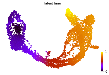
#latent_time
scv.tl.latent_time(adata)
computing latent time using root_cells as prior
    finished (0:00:02) --> added
    'latent_time', shared time (adata.obs)
scv.pl.scatter(adata, color='latent_time', color_map='gnuplot', size=80)
top_genes = adata.var['fit_likelihood'].sort_values(ascending=False).index[:300]
top_genes
Index(['Pcsk2', 'Dcdc2a', 'Ank', 'Gng12', 'Top2a', 'Pak3', 'Tmem163', 'Nfib',
       'Pim2', 'Smoc1',
       ...
       'Cyr61', 'Ptprn2', 'Rpa2', 'Nit2', 'Cdc20', 'Hmmr', 'Ankrd12', 'Itpr1',
       'Auts2', 'Mdfi'],
      dtype='object', name='index', length=300)
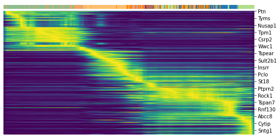
scv.pl.heatmap(adata, var_names=top_genes, sortby='latent_time', col_color='clusters', n_convolve=100)
top = df['fit_likelihood'].sort_values(ascending=False).index[:300]
top
Index(['Pcsk2', 'Dcdc2a', 'Ank', 'Gng12', 'Top2a', 'Pak3', 'Tmem163', 'Nfib',
       'Pim2', 'Smoc1',
       ...
       'Trp53inp2', 'Ccnb1', 'Atp2a2', 'Dtl', 'Kmt2a', 'Emb', 'Rcan2',
       'Gm28172', 'Rab3b', 'Gk'],
      dtype='object', name='index', length=300)
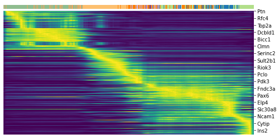
scv.pl.heatmap(adata, var_names=top, sortby='latent_time', col_color='clusters', n_convolve=100)
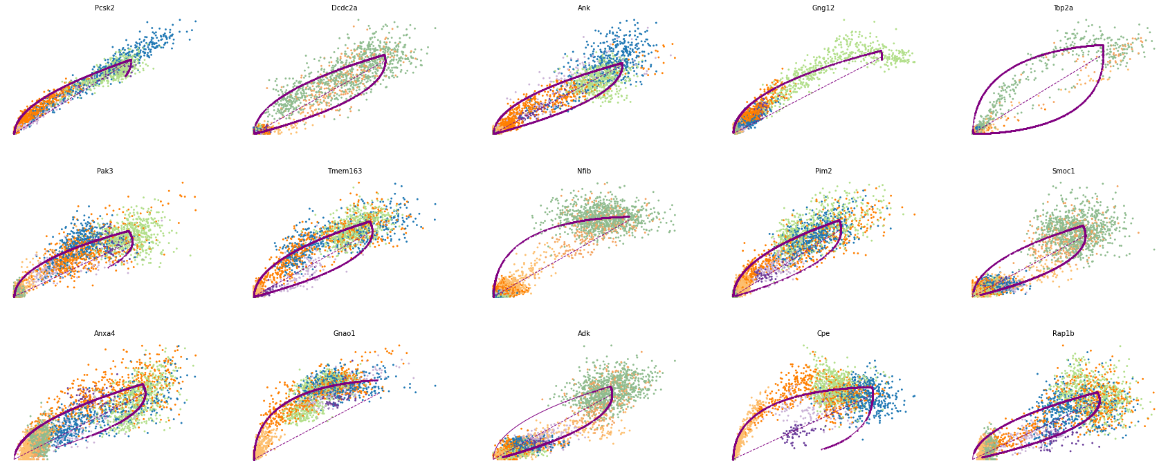
# 驱动基因
top_genes = adata.var['fit_likelihood'].sort_values(ascending=False).index
scv.pl.scatter(adata, basis=top_genes[:15], ncols=5, frameon=False)
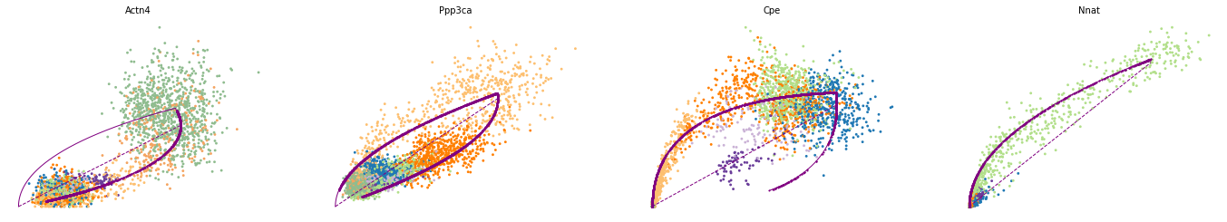
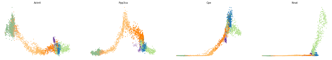
var_names = ['Actn4', 'Ppp3ca', 'Cpe', 'Nnat']
scv.pl.scatter(adata, var_names, frameon=False)
scv.pl.scatter(adata, x='latent_time', y=var_names, frameon=False)
#特定于簇的最高似然基因
scv.tl.rank_dynamical_genes(adata, groupby='clusters')
df = scv.get_df(adata, 'rank_dynamical_genes/names')
df.head(5)
ranking genes by cluster-specific likelihoods
    finished (0:00:05) --> added
    'rank_dynamical_genes', sorted scores by group ids (adata.uns)
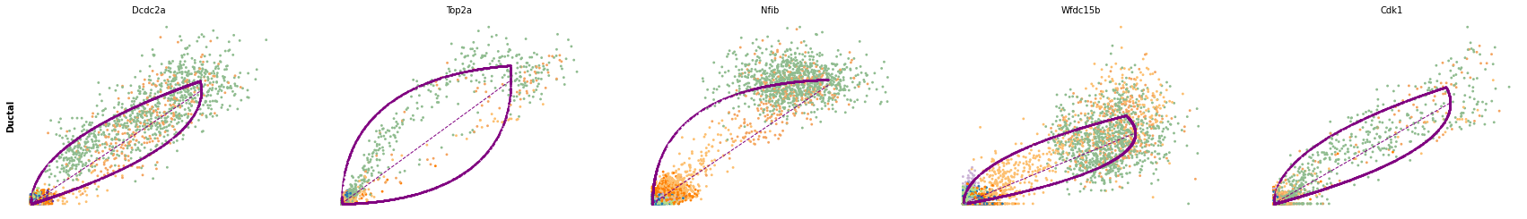
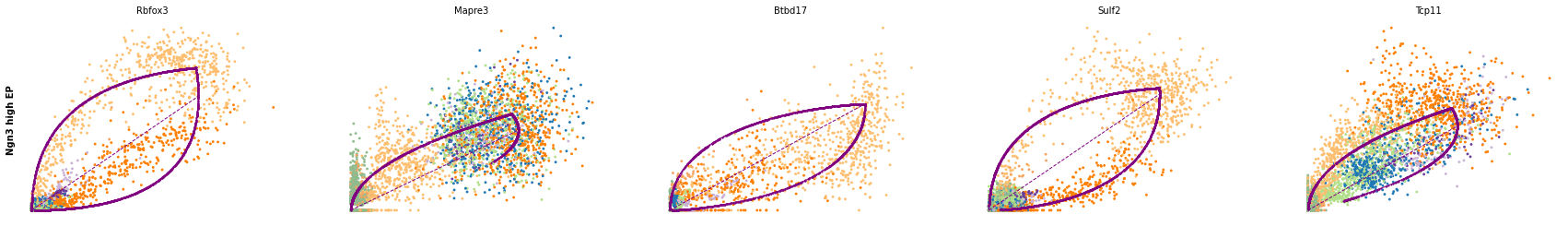
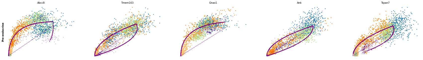
| Ductal | Ngn3 low EP | Ngn3 high EP | Pre-endocrine | Beta | Alpha | Delta | Epsilon | |
|---|---|---|---|---|---|---|---|---|
| 0 | Dcdc2a | Dcdc2a | Rbfox3 | Abcc8 | Pcsk2 | Cpe | Pcsk2 | Tox3 |
| 1 | Top2a | Adk | Mapre3 | Tmem163 | Ank | Gnao1 | Rap1b | Rnf130 |
| 2 | Nfib | Mki67 | Btbd17 | Gnao1 | Tmem163 | Pak3 | Pak3 | Meis2 |
| 3 | Wfdc15b | Rap1gap2 | Sulf2 | Ank | Tspan7 | Pim2 | Abcc8 | Adk |
| 4 | Cdk1 | Top2a | Tcp11 | Tspan7 | Map1b | Map1b | Slc7a14 | Rap1gap2 |
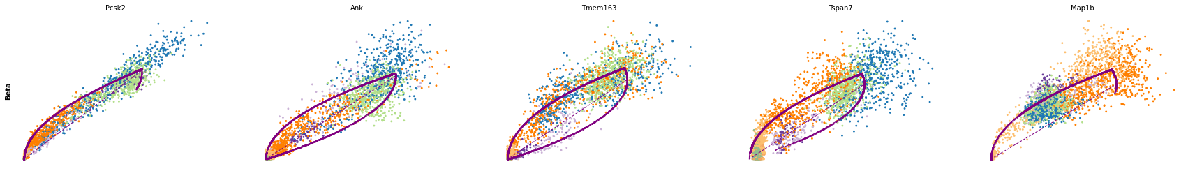
for cluster in ['Ductal', 'Ngn3 high EP', 'Pre-endocrine', 'Beta']:
    scv.pl.scatter(adata, df[cluster][:5], ylabel=cluster, frameon=False)
df = scv.get_df(adata, 'rank_dynamical_genes/scores')
df.head(5)
| Ductal | Ngn3 low EP | Ngn3 high EP | Pre-endocrine | Beta | Alpha | Delta | Epsilon | |
|---|---|---|---|---|---|---|---|---|
| 0 | 0.59 | 0.59 | 0.53 | 0.73 | 0.90 | 0.61 | 0.96 | 0.61 |
| 1 | 0.56 | 0.53 | 0.50 | 0.54 | 0.70 | 0.57 | 0.70 | 0.61 |
| 2 | 0.56 | 0.51 | 0.47 | 0.53 | 0.59 | 0.54 | 0.67 | 0.59 |
| 3 | 0.50 | 0.50 | 0.46 | 0.53 | 0.59 | 0.54 | 0.62 | 0.57 |
| 4 | 0.49 | 0.49 | 0.45 | 0.51 | 0.57 | 0.51 | 0.60 | 0.55 |
[参考链接1](https://scvelo.readthedocs.io/DynamicalModeling.html)
[参考链接2](https://www.bilibili.com/read/cv7764833/)