本笔记本通过一个示例说明如何在非rgb数据上使用DenseCRFs。同时,它将解释基本概念并通过一个示例进行演示,因此即使您正在处理RGB数据,它也可能是有用的,不过也请查看PyDenseCRF's README !
在jupyter notebook上运行https://github.com/lucasb-eyer/pydensecrf/tree/master/examples/Non RGB Example.ipynb
Basic setup
先导入:
import pydensecrf.densecrf as dcrf
from pydensecrf.utils import unary_from_softmax, create_pairwise_bilateral
设置画图风格:
import numpy as np
import matplotlib.pyplot as plt

%matplotlib inline

plt.rcParams['image.interpolation'] = 'nearest' #设置插入风格
plt.rcParams['image.cmap'] = 'gray' #设置颜色风格
Unary Potential一元势
一元势由每个像素的类概率组成。这可以来自任何类型的模型,如随机森林或深度神经网络的softmax。
1)Create unary potential
补充:scipy.stats.multivariate_normal的使用
1.得到x,y的取值
from scipy.stats import multivariate_normal

H, W, NLABELS = 400, 512, 2

# This creates a gaussian blob...
a = np.mgrid[0:H, 0:W] #(2,400,512) #得到x,y的取值
a,a.shape
返回:
(array([[[  0,   0,   0, ...,   0,   0,   0],
         [  1,   1,   1, ...,   1,   1,   1],
         [  2,   2,   2, ...,   2,   2,   2],
         ...,
         [397, 397, 397, ..., 397, 397, 397],
         [398, 398, 398, ..., 398, 398, 398],
         [399, 399, 399, ..., 399, 399, 399]],

        [[  0,   1,   2, ..., 509, 510, 511],
         [  0,   1,   2, ..., 509, 510, 511],
         [  0,   1,   2, ..., 509, 510, 511],
         ...,
         [  0,   1,   2, ..., 509, 510, 511],
         [  0,   1,   2, ..., 509, 510, 511],
         [  0,   1,   2, ..., 509, 510, 511]]]), (2, 400, 512))
2.得到点(x,y)的值
pos = np.stack(a, axis=2) #得到(x,y)点的值
pos,pos.shape
返回:
(array([[[  0,   0],
         [  0,   1],
         [  0,   2],
         ...,
         [  0, 509],
         [  0, 510],
         [  0, 511]],

        [[  1,   0],
         [  1,   1],
         [  1,   2],
         ...,
         [  1, 509],
         [  1, 510],
         [  1, 511]],

        [[  2,   0],
         [  2,   1],
         [  2,   2],
         ...,
         [  2, 509],
         [  2, 510],
         [  2, 511]],

        ...,

        [[397,   0],
         [397,   1],
         [397,   2],
         ...,
         [397, 509],
         [397, 510],
         [397, 511]],

        [[398,   0],
         [398,   1],
         [398,   2],
         ...,
         [398, 509],
         [398, 510],
         [398, 511]],

        [[399,   0],
         [399,   1],
         [399,   2],
         ...,
         [399, 509],
         [399, 510],
         [399, 511]]]), (400, 512, 2))
3.得到概率值:
#mean=[200, 256], cov=12800,12800的单位乘作为协方差矩阵
rv = multivariate_normal([H//2, W//2], (H//4)*(W//4))
probs = rv.pdf(pos)
probs,probs.shape
返回:
(array([[2.01479637e-07, 2.05541767e-07, 2.09669414e-07, ...,
         2.13863243e-07, 2.09669414e-07, 2.05541767e-07],
        [2.04644486e-07, 2.08770423e-07, 2.12962908e-07, ...,
         2.17222613e-07, 2.12962908e-07, 2.08770423e-07],
        [2.07842810e-07, 2.12033230e-07, 2.16291237e-07, ...,
         2.20617517e-07, 2.16291237e-07, 2.12033230e-07],
        ...,
        [2.11074628e-07, 2.15330207e-07, 2.19654423e-07, ...,
         2.24047973e-07, 2.19654423e-07, 2.15330207e-07],
        [2.07842810e-07, 2.12033230e-07, 2.16291237e-07, ...,
         2.20617517e-07, 2.16291237e-07, 2.12033230e-07],
        [2.04644486e-07, 2.08770423e-07, 2.12962908e-07, ...,
         2.17222613e-07, 2.12962908e-07, 2.08770423e-07]]), (400, 512))
4.将概率值进行处理集中到[0.4,0.6]区间中
先将值集中到[0,1]区间中
# ...which we project into the range [0.4, 0.6]
probs = (probs-probs.min()) / (probs.max()-probs.min())
probs, probs.shape
返回:
(array([[0.        , 0.00033208, 0.00066951, ..., 0.00101235, 0.00066951,
         0.00033208],
        [0.00025872, 0.00059602, 0.00093875, ..., 0.00128698, 0.00093875,
         0.00059602],
        [0.00052019, 0.00086275, 0.00121084, ..., 0.00156451, 0.00121084,
         0.00086275],
        ...,
        [0.00078439, 0.00113228, 0.00148578, ..., 0.00184495, 0.00148578,
         0.00113228],
        [0.00052019, 0.00086275, 0.00121084, ..., 0.00156451, 0.00121084,
         0.00086275],
        [0.00025872, 0.00059602, 0.00093875, ..., 0.00128698, 0.00093875,
         0.00059602]]), (400, 512))
再将其集中到[0.4,0.6]区间中,0.5 + 0.2 * (probs-0.5)等价于0.4+0.2*probs,而此时的probs为[0,1]区间中的值:
probs = 0.5 + 0.2 * (probs-0.5) #此时probs.shape为(400, 512)
probs, probs.shape #将最终的概率结果的值集中在[0.4, 0.6]区间中
返回:
(array([[0.4       , 0.40006642, 0.4001339 , ..., 0.40020247, 0.4001339 ,
         0.40006642],
        [0.40005174, 0.4001192 , 0.40018775, ..., 0.4002574 , 0.40018775,
         0.4001192 ],
        [0.40010404, 0.40017255, 0.40024217, ..., 0.4003129 , 0.40024217,
         0.40017255],
        ...,
        [0.40015688, 0.40022646, 0.40029716, ..., 0.40036899, 0.40029716,
         0.40022646],
        [0.40010404, 0.40017255, 0.40024217, ..., 0.4003129 , 0.40024217,
         0.40017255],
        [0.40005174, 0.4001192 , 0.40018775, ..., 0.4002574 , 0.40018775,
         0.4001192 ]]), (400, 512))
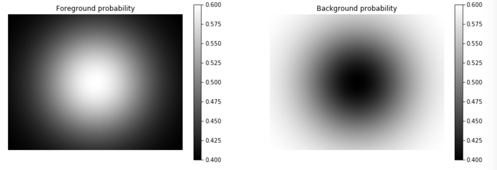
5.一份数据已经准备好了,要复制生成一个效果相反的数据:
# 第一个维度需要等于类的数量,这里设置两个类,为2
# 让我们有一个"foreground"和一个"background"类
#因此,复制高斯blob,但倒置它去创建与“background”类的概率是相反的“foreground”类。
#np.tile(a,(m,n)):即是把a数组里面的元素复制n次放进一个数组c中,然后再把数组c复制m次放进一个数组b中
#np.tile(a,(2,3)) #将a数组重复3次形成2行的数组
#np.newaxis为多维数组增加一个轴
#probs[np.newaxis,:,:].shape为(1, 400, 512)
probs = np.tile(probs[np.newaxis,:,:],(2,1,1))#此时probs.shape为(2, 400, 512)
probs[1,:,:] = 1 - probs[0,:,:] #得到相反的值
probs,probs.shape
返回:
(array([[[0.4       , 0.40006642, 0.4001339 , ..., 0.40020247,
          0.4001339 , 0.40006642],
         [0.40005174, 0.4001192 , 0.40018775, ..., 0.4002574 ,
          0.40018775, 0.4001192 ],
         [0.40010404, 0.40017255, 0.40024217, ..., 0.4003129 ,
          0.40024217, 0.40017255],
         ...,
         [0.40015688, 0.40022646, 0.40029716, ..., 0.40036899,
          0.40029716, 0.40022646],
         [0.40010404, 0.40017255, 0.40024217, ..., 0.4003129 ,
          0.40024217, 0.40017255],
         [0.40005174, 0.4001192 , 0.40018775, ..., 0.4002574 ,
          0.40018775, 0.4001192 ]],

        [[0.6       , 0.59993358, 0.5998661 , ..., 0.59979753,
          0.5998661 , 0.59993358],
         [0.59994826, 0.5998808 , 0.59981225, ..., 0.5997426 ,
          0.59981225, 0.5998808 ],
         [0.59989596, 0.59982745, 0.59975783, ..., 0.5996871 ,
          0.59975783, 0.59982745],
         ...,
         [0.59984312, 0.59977354, 0.59970284, ..., 0.59963101,
          0.59970284, 0.59977354],
         [0.59989596, 0.59982745, 0.59975783, ..., 0.5996871 ,
          0.59975783, 0.59982745],
         [0.59994826, 0.5998808 , 0.59981225, ..., 0.5997426 ,
          0.59981225, 0.5998808 ]]]), (2, 400, 512))
6.最终的代码为:
from scipy.stats import multivariate_normal

H, W, NLABELS = 400, 512, 2

# This creates a gaussian blob...
pos = np.stack(np.mgrid[0:H, 0:W], axis=2)

rv = multivariate_normal([H//2, W//2], (H//4)*(W//4))
probs = rv.pdf(pos)

# ...which we project into the range [0.4, 0.6]
probs = (probs-probs.min()) / (probs.max()-probs.min())
probs = 0.5 + 0.2 * (probs-0.5) #此时probs.shape为(400, 512)

# 第一个维度需要等于类的数量
# 让我们有一个"foreground"和一个"background"类
#因此,复制高斯blob,但倒置它去创建与“background”类的概率是相反的“foreground”类。
#np.tile(a,(m,n)):即是把a数组里面的元素复制n次放进一个数组c中,然后再把数组c复制m次放进一个数组b中
#np.tile(a,(2,3)) #将a数组重复3次形成2行的数组
#np.newaxis为多维数组增加一个轴
#probs[np.newaxis,:,:].shape为(1, 400, 512)
probs = np.tile(probs[np.newaxis,:,:],(2,1,1))#此时probs.shape为(2, 400, 512)
probs[1,:,:] = 1 - probs[0,:,:] #得到相反的值

# Let's have a look:
plt.figure(figsize=(15,5))
plt.subplot(1,2,1); plt.imshow(probs[0,:,:]); plt.title('Foreground probability'); plt.axis('off'); plt.colorbar();
plt.subplot(1,2,2); plt.imshow(probs[1,:,:]); plt.title('Background probability'); plt.axis('off'); plt.colorbar();
返回:
2)Run inference with unary potential 使用一元势运行推理
我们已经可以运行一个只有一元势的DenseCRF。这不是一个好主意,但我们可以做到:
1.unary_from_softmax函数的作用
将softmax类概率转换为一元势(每个节点的NLL)。
即我们之前先对图片使用训练好的网络预测得到最终经过softmax函数得到的分类结果,这里需要将这个结果转成一元势
参数
- sm: numpy.array ,第一个维度是类的softmax的输出,其他所有维度都是flattend。这意味着“sm.shape[0] == n_classes”。
- scale: float,softmax输出的确定性(默认为None),需要值在(0,1]。如果不为None,则softmax输出被缩放到从[0,scale]概率的范围。
- clip: float,将概率裁剪到的最小值。这是因为一元函数是概率的负对数,而log(0) = inf,所以我们需要把0概率裁剪成正的值。
在这里因为scale=None,clip=None,所以这个函数的作用其实只进行了下面的操作:
-np.log(sm).reshape([num_cls, -1]).astype(np.float32)
对值取负对数,并将结果变为(2, 204800)大小,进行了flatten操作,将图片压扁了:
# Inference without pair-wise terms
#设置固定的一元势
from pydensecrf.utils import unary_from_softmax
U = unary_from_softmax(probs)  # note: num classes is first dim,类别在第一维
U,U.shape
返回:
(array([[0.91629076, 0.9161247 , 0.915956  , ..., 0.91564745, 0.9158215 ,
         0.9159928 ],
        [0.51082563, 0.5109363 , 0.5110488 , ..., 0.5112547 , 0.5111386 ,
         0.5110243 ]], dtype=float32), (2, 204800))
此时的值就是一元势了
d = dcrf.DenseCRF2D(W, H, NLABELS)
d.setUnaryEnergy(U)

# Run inference for 10 iterations,10次迭代
Q_unary = d.inference(10)

# Q现在是近似后验,我们可以用argmax得到一个MAP估计值。
#np.argmax得到Q_unary列方向上的最大值的索引
map_soln_unary = np.argmax(Q_unary, axis=0)#此时形式为(204800,)
map_soln_unary,map_soln_unary.shape
返回:
(array([1, 1, 1, ..., 1, 1, 1]), (204800,))
# 不幸的是,DenseCRF把所有东西都压扁了,所以把它恢复到图片形式。
map_soln_unary = map_soln_unary.reshape((H,W)) #重新变为(400, 512))
map_soln_unary,map_soln_unary.shape
返回:
(array([[1, 1, 1, ..., 1, 1, 1],
        [1, 1, 1, ..., 1, 1, 1],
        [1, 1, 1, ..., 1, 1, 1],
        ...,
        [1, 1, 1, ..., 1, 1, 1],
        [1, 1, 1, ..., 1, 1, 1],
        [1, 1, 1, ..., 1, 1, 1]]), (400, 512))
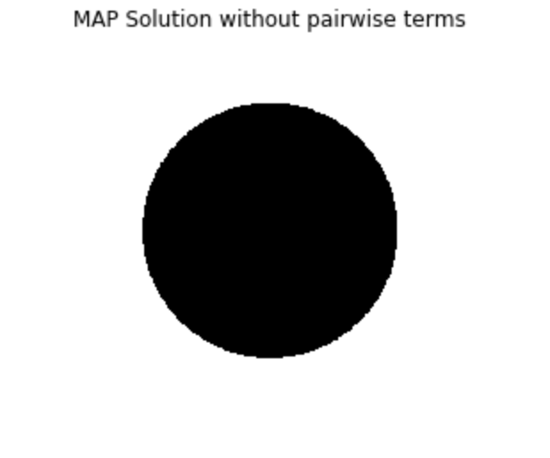
总的代码为:
# Inference without pair-wise terms
U = unary_from_softmax(probs)  # note: num classes is first dim
d = dcrf.DenseCRF2D(W, H, NLABELS)
d.setUnaryEnergy(U)

# Run inference for 10 iterations,10次迭代
Q_unary = d.inference(10)

# Q现在是近似后验,我们可以用argmax得到一个MAP估计值。
#np.argmax得到Q_unary列方向上的最大值的索引
map_soln_unary = np.argmax(Q_unary, axis=0)#此时形式为(204800,)

# 不幸的是,DenseCRF把所有东西都压扁了,所以把它恢复到图片形式。
map_soln_unary = map_soln_unary.reshape((H,W))#重新变为(400, 512))

# And let's have a look.
plt.imshow(map_soln_unary); plt.axis('off'); plt.title('MAP Solution without pairwise terms');
返回:

因为设置了颜色为gray,实际结果为:
Pairwise terms二元
DenseCRFs的全部意义在于使用某种形式的内容来平滑预测。这是通过“成对”术语来实现的,“成对”术语编码元素之间的关系。
1)Add (non-RGB) pairwise term
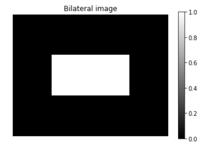
例如,在图像处理中,一个流行的成对关系是“双边”(bilateral)关系,它大致表示颜色相似或位置相似的像素可能属于同一个类。
NCHAN=1 #通道为1,non-RGB

#创造简单的双边图象。
#注意,我们将通道维度放在最后,但我们也可以将它作为第一个维度,只要将chdim参数进一步更改为0。
img = np.zeros((H,W,NCHAN), np.uint8)
img[H//3:2*H//3,W//4:3*W//4,:] = 1 #使得[133:266,128:384,:]内的值为1,下面画为白色

plt.imshow(img[:,:,0]); plt.title('Bilateral image'); plt.axis('off'); plt.colorbar();
返回:
2.create_pairwise_bilateral函数的作用
创造成对双边势的Util函数。这适用于所有的图像尺寸。对于2D情况,与“densecrf2 . addpairwisebilateral”函数效果相同。
参数:
- sdims: list or tuple,每个维度的比例因子。这在DenseCRF2D.addPairwiseBilateral中称为“sxy”。
- schan: list or tuple,图像中每个通道的比例因子。这在DenseCRF2D.addPairwiseBilateral中称为“srgb”。
- img: numpy.array,输入的图像
- chdim: int, 可选。这指定了通道维度在图像中的位置。例如,' chdim=2 '用于大小为(240,300,3)的RGB图像,说明其通道3值放在维度2上(维度从0开始)。如果图像没有通道尺寸(例如只有一个通道),则使用' chdim=-1 '。
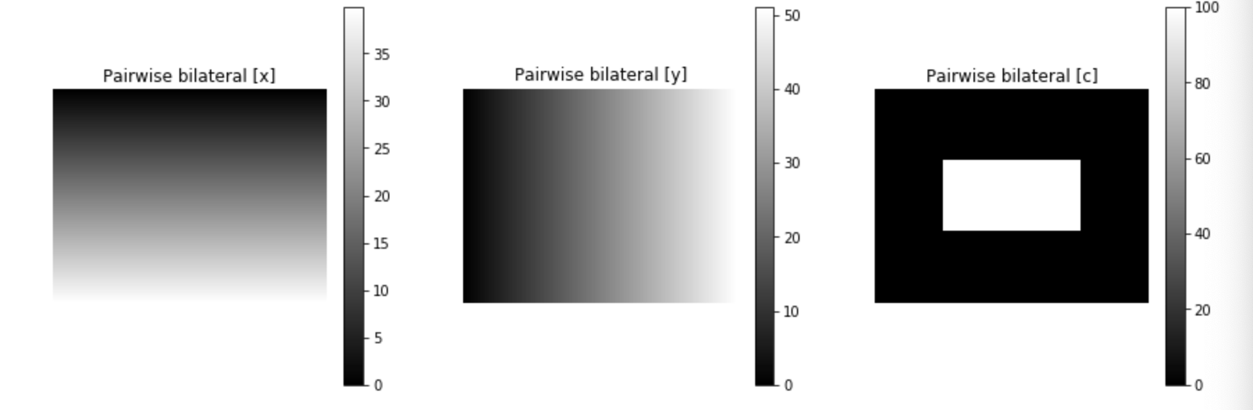
#从上图中创建成对的双边术语。
#这两个' s{dims,chan} '参数是模型超参数,分别定义了位置的强度和图像内容的双边参数。
#将通道为1的图变为了通道为3的图
pairwise_energy = create_pairwise_bilateral(sdims=(10,10), schan=(0.01,), img=img, chdim=2) #其shape为(3, 204800)

#pairwise_energy现在包含的维度和DenseCRF的特性一样多,在本例中是3:(x,y,channel1)
img_en = pairwise_energy.reshape((-1, H, W))  # Reshape just for plotting,为了画图

#下面将三个通道对应的图画出来
plt.figure(figsize=(15,5))
plt.subplot(1,3,1); plt.imshow(img_en[0]); plt.title('Pairwise bilateral [x]'); plt.axis('off'); plt.colorbar();
plt.subplot(1,3,2); plt.imshow(img_en[1]); plt.title('Pairwise bilateral [y]'); plt.axis('off'); plt.colorbar();
plt.subplot(1,3,3); plt.imshow(img_en[2]); plt.title('Pairwise bilateral [c]'); plt.axis('off'); plt.colorbar();
返回:
2)Run inference of complete DenseCRF
现在我们可以创建一个包含一元势和成对势的dense CRF ,并对其进行推理以得到最终结果。
d = dcrf.DenseCRF2D(W, H, NLABELS)
d.setUnaryEnergy(U) #设置一元势
#添加二元势
d.addPairwiseEnergy(pairwise_energy, compat=10)  # `compat` is the "strength" of this potential.

#这一次,让我们自己分步骤进行推理,这样我们就可以查看中间解,并监视KL-divergence,它表明我们收敛得有多好。
#PyDenseCRF还要求我们跟踪计算所需的两个临时缓冲区,tmp1, tmp2。
Q, tmp1, tmp2 = d.startInference()
for _ in range(5): #迭代5次后,查看结果
    d.stepInference(Q, tmp1, tmp2)
kl1 = d.klDivergence(Q) / (H*W)
map_soln1 = np.argmax(Q, axis=0).reshape((H,W))

for _ in range(20):
    d.stepInference(Q, tmp1, tmp2)
kl2 = d.klDivergence(Q) / (H*W)
map_soln2 = np.argmax(Q, axis=0).reshape((H,W))

for _ in range(50):
    d.stepInference(Q, tmp1, tmp2)
kl3 = d.klDivergence(Q) / (H*W)
map_soln3 = np.argmax(Q, axis=0).reshape((H,W))

img_en = pairwise_energy.reshape((-1, H, W))  # Reshape just for plotting
plt.figure(figsize=(15,5))
plt.subplot(1,3,1); plt.imshow(map_soln1);
plt.title('MAP Solution with DenseCRF
(5 steps, KL={:.2f})'.format(kl1)); plt.axis('off');
plt.subplot(1,3,2); plt.imshow(map_soln2);
plt.title('MAP Solution with DenseCRF
(20 steps, KL={:.2f})'.format(kl2)); plt.axis('off');
plt.subplot(1,3,3); plt.imshow(map_soln3);
plt.title('MAP Solution with DenseCRF
(50 steps, KL={:.2f})'.format(kl3)); plt.axis('off');
返回:

这个不太好看出效果,下面:
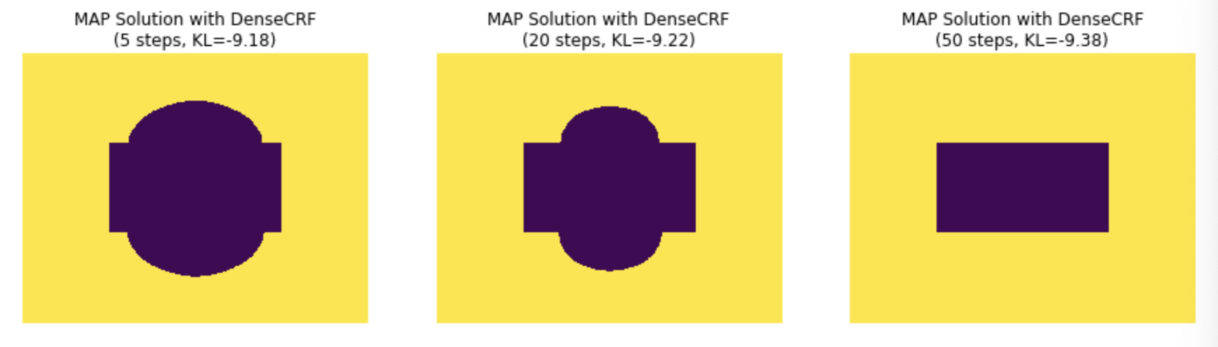
可见50次迭代后效果很好