
The 9 Deep Learning Papers You Need To Know About (Understanding CNNs Part 3)
Introduction
In this post, we’ll go into summarizing a lot of the new and important developments in the field of computer vision and convolutional neural networks. We’ll look at some of the most important papers that have been published over the last 5 years and discuss why they’re so important. The first half of the list (AlexNet to ResNet) deals with advancements in general network architecture, while the second half is just a collection of interesting papers in other subareas.
AlexNet (2012)
The one that started it all (Though some may say that Yann LeCun’s paper in 1998 was the real pioneering publication). This paper, titled “ImageNet Classification with Deep Convolutional Networks”, has been cited a total of 6,184 times and is widely regarded as one of the most influential publications in the field. Alex Krizhevsky, Ilya Sutskever, and Geoffrey Hinton created a “large, deep convolutional neural network” that was used to win the 2012 ILSVRC (ImageNet Large-Scale Visual Recognition Challenge). For those that aren’t familiar, this competition can be thought of as the annual Olympics of computer vision, where teams from across the world compete to see who has the best computer vision model for tasks such as classification, localization, detection, and more. 2012 marked the first year where a CNN was used to achieve a top 5 test error rate of 15.4% (Top 5 error is the rate at which, given an image, the model does not output the correct label with its top 5 predictions). The next best entry achieved an error of 26.2%, which was an astounding improvement that pretty much shocked the computer vision community. Safe to say, CNNs became household names in the competition from then on out.
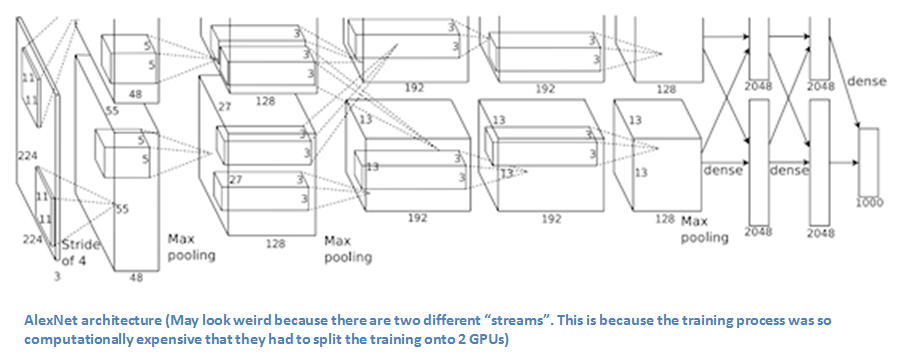
In the paper, the group discussed the architecture of the network (which was called AlexNet). They used a relatively simple layout, compared to modern architectures. The network was made up of 5 conv layers, max-pooling layers, dropout layers, and 3 fully connected layers. The network they designed was used for classification with 1000 possible categories.
Main Points
- Trained the network on ImageNet data, which contained over 15 million annotated images from a total of over 22,000 categories.
- Used ReLU for the nonlinearity functions (Found to decrease training time as ReLUs are several times faster than the conventional tanh function).
- Used data augmentation techniques that consisted of image translations, horizontal reflections, and patch extractions.
- Implemented dropout layers in order to combat the problem of overfitting to the training data.
- Trained the model using batch stochastic gradient descent, with specific values for momentum and weight decay.
- Trained on two GTX 580 GPUs for five to six days.
Why It’s Important
The neural network developed by Krizhevsky, Sutskever, and Hinton in 2012 was the coming out party for CNNs in the computer vision community. This was the first time a model performed so well on a historically difficult ImageNet dataset. Utilizing techniques that are still used today, such as data augmentation and dropout, this paper really illustrated the benefits of CNNs and backed them up with record breaking performance in the competition.
ZF Net (2013)
With AlexNet stealing the show in 2012, there was a large increase in the number of CNN models submitted to ILSVRC 2013. The winner of the competition that year was a network built by Matthew Zeiler and Rob Fergus from NYU. Named ZF Net, this model achieved an 11.2% error rate. This architecture was more of a fine tuning to the previous AlexNet structure, but still developed some very keys ideas about improving performance. Another reason this was such a great paper is that the authors spent a good amount of time explaining a lot of the intuition behind ConvNets and showing how to visualize the filters and weights correctly.
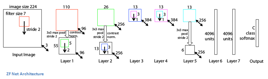
In this paper titled “Visualizing and Understanding Convolutional Neural Networks”, Zeiler and Fergus begin by discussing the idea that this renewed interest in CNNs is due to the accessibility of large training sets and increased computational power with the usage of GPUs. They also talk about the limited knowledge that researchers had on inner mechanisms of these models, saying that without this insight, the “development of better models is reduced to trial and error”. While we do currently have a better understanding than 3 years ago, this still remains an issue for a lot of researchers! The main contributions of this paper are details of a slightly modified AlexNet model and a very interesting way of visualizing feature maps.
Main Points
- Very similar architecture to AlexNet, except for a few minor modifications.
- AlexNet trained on 15 million images, while ZF Net trained on only 1.3 million images.
- Instead of using 11x11 sized filters in the first layer (which is what AlexNet implemented), ZF Net used filters of size 7x7 and a decreased stride value. The reasoning behind this modification is that a smaller filter size in the first conv layer helps retain a lot of original pixel information in the input volume. A filtering of size 11x11 proved to be skipping a lot of relevant information, especially as this is the first conv layer.
- As the network grows, we also see a rise in the number of filters used.
- Used ReLUs for their activation functions, cross-entropy loss for the error function, and trained using batch stochastic gradient descent.
- Trained on a GTX 580 GPU for twelve days.
- Developed a visualization technique named Deconvolutional Network, which helps to examine different feature activations and their relation to the input space. Called “deconvnet” because it maps features to pixels (the opposite of what a convolutional layer does).
DeConvNet
The basic idea behind how this works is that at every layer of the trained CNN, you attach a “deconvnet” which has a path back to the image pixels. An input image is fed into the CNN and activations are computed at each level. This is the forward pass. Now, let’s say we want to examine the activations of a certain feature in the 4th conv layer. We would store the activations of this one feature map, but set all of the other activations in the layer to 0, and then pass this feature map as the input into the deconvnet. This deconvnet has the same filters as the original CNN. This input then goes through a series of unpool (reverse maxpooling), rectify, and filter operations for each preceding layer until the input space is reached.
The reasoning behind this whole process is that we want to examine what type of structures excite a given feature map. Let’s look at the visualizations of the first and second layers.
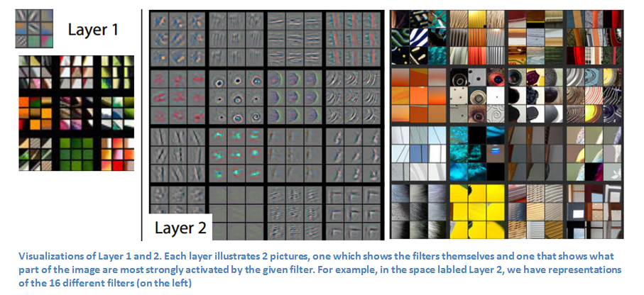
Like we discussed in Part 1, the first layer of your ConvNet is always a low level feature detector that will detect simple edges or colors in this particular case. We can see that with the second layer, we have more circular features that are being detected. Let’s look at layers 3, 4, and 5.
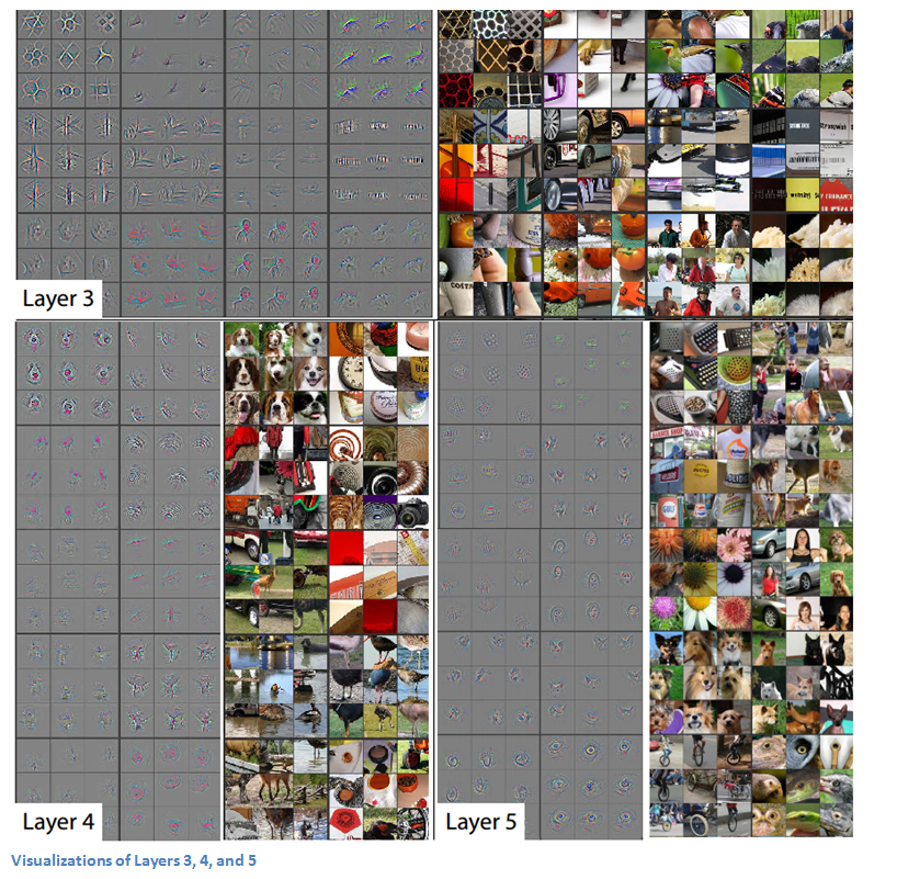
These layers show a lot more of the higher level features such as dogs’ faces or flowers. One thing to note is that as you may remember, after the first conv layer, we normally have a pooling layer that downsamples the image (for example, turns a 32x32x3 volume into a 16x16x3 volume). The effect this has is that the 2nd layer has a broader scope of what it can see in the original image. For more info on deconvnet or the paper in general, check out Zeiler himself presenting on the topic.
Why It’s Important
ZF Net was not only the winner of the competition in 2013, but also provided great intuition as to the workings on CNNs and illustrated more ways to improve performance. The visualization approach described helps not only to explain the inner workings of CNNs, but also provides insight for improvements to network architectures. The fascinating deconv visualization approach and occlusion experiments make this one of my personal favorite papers.
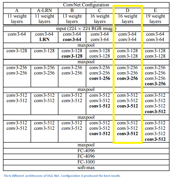
VGG Net (2014)
Simplicity and depth. That’s what a model created in 2014 (weren’t the winners of ILSVRC 2014) best utilized with its 7.3% error rate. Karen Simonyan and Andrew Zisserman of the University of Oxford created a 19 layer CNN that strictly used 3x3 filters with stride and pad of 1, along with 2x2 maxpooling layers with stride 2. Simple enough right?
Main Points
- The use of only 3x3 sized filters is quite different from AlexNet’s 11x11 filters in the first layer and ZF Net’s 7x7 filters. The authors’ reasoning is that the combination of two 3x3 conv layers has an effective receptive field of 5x5. This in turn simulates a larger filter while keeping the benefits of smaller filter sizes. One of the benefits is a decrease in the number of parameters. Also, with two conv layers, we’re able to use two ReLU layers instead of one.
- 3 conv layers back to back have an effective receptive field of 7x7.
- As the spatial size of the input volumes at each layer decrease (result of the conv and pool layers), the depth of the volumes increase due to the increased number of filters as you go down the network.
- Interesting to notice that the number of filters doubles after each maxpool layer. This reinforces the idea of shrinking spatial dimensions, but growing depth.
- Worked well on both image classification and localization tasks. The authors used a form of localization as regression (see page 10 of the paper for all details).
- Built model with the Caffe toolbox.
- Used scale jittering as one data augmentation technique during training.
- Used ReLU layers after each conv layer and trained with batch gradient descent.
- Trained on 4 Nvidia Titan Black GPUs for two to three weeks.
Why It’s Important
VGG Net is one of the most influential papers in my mind because it reinforced the notion that convolutional neural networks have to have a deep network of layers in order for this hierarchical representation of visual data to work. Keep it deep. Keep it simple.
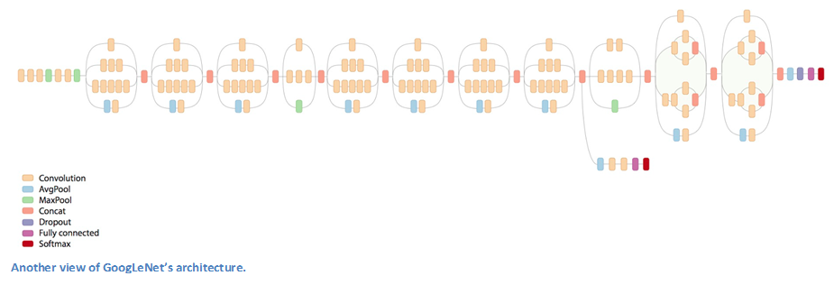
GoogLeNet (2015)
You know that idea of simplicity in network architecture that we just talked about? Well, Google kind of threw that out the window with the introduction of the Inception module. GoogLeNet is a 22 layer CNN and was the winner of ILSVRC 2014 with a top 5 error rate of 6.7%. To my knowledge, this was one of the first CNN architectures that really strayed from the general approach of simply stacking conv and pooling layers on top of each other in a sequential structure. The authors of the paper also emphasized that this new model places notable consideration on memory and power usage (Important note that I sometimes forget too: Stacking all of these layers and adding huge numbers of filters has a computational and memory cost, as well as an increased chance of overfitting).
Inception Module
When we first take a look at the structure of GoogLeNet, we notice immediately that not everything is happening sequentially, as seen in previous architectures. We have pieces of the network that are happening in parallel.
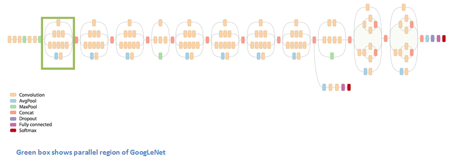
This box is called an Inception module. Let’s take a closer look at what it’s made of.
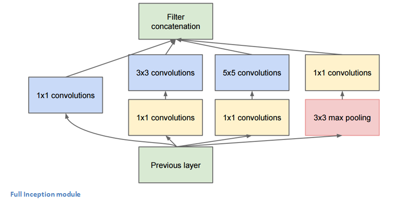
The bottom green box is our input and the top one is the output of the model (Turning this picture right 90 degrees would let you visualize the model in relation to the last picture which shows the full network). Basically, at each layer of a traditional ConvNet, you have to make a choice of whether to have a pooling operation or a conv operation (there is also the choice of filter size). What an Inception module allows you to do is perform all of these operations in parallel. In fact, this was exactly the “naïve” idea that the authors came up with.
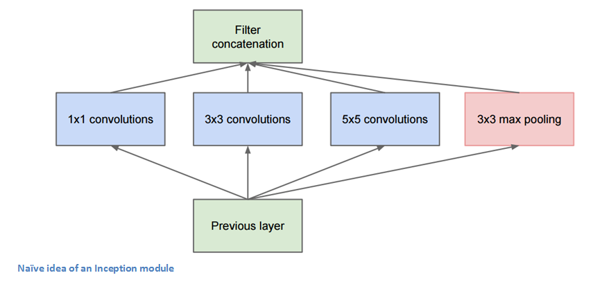
Now, why doesn’t this work? It would lead to way too many outputs. We would end up with an extremely large depth channel for the output volume. The way that the authors address this is by adding 1x1 conv operations before the 3x3 and 5x5 layers. The 1x1 convolutions (or network in network layer) provide a method of dimensionality reduction. For example, let’s say you had an input volume of 100x100x60 (This isn’t necessarily the dimensions of the image, just the input to any layer of the network). Applying 20 filters of 1x1 convolution would allow you to reduce the volume to 100x100x20. This means that the 3x3 and 5x5 convolutions won’t have as large of a volume to deal with. This can be thought of as a “pooling of features” because we are reducing the depth of the volume, similar to how we reduce the dimensions of height and width with normal maxpooling layers. Another note is that these 1x1 conv layers are followed by ReLU units which definitely can’t hurt (See Aaditya Prakash’s great post for more info on the effectiveness of 1x1 convolutions). Check out this video for a great visualization of the filter concatenation at the end.
You may be asking yourself “How does this architecture help?”. Well, you have a module that consists of a network in network layer, a medium sized filter convolution, a large sized filter convolution, and a pooling operation. The network in network conv is able to extract information about the very fine grain details in the volume, while the 5x5 filter is able to cover a large receptive field of the input, and thus able to extract its information as well. You also have a pooling operation that helps to reduce spatial sizes and combat overfitting. On top of all of that, you have ReLUs after each conv layer, which help improve the nonlinearity of the network. Basically, the network is able to perform the functions of these different operations while still remaining computationally considerate. The paper does also give more of a high level reasoning that involves topics like sparsity and dense connections (read Sections 3 and 4 of the paper. Still not totally clear to me, but if anybody has any insights, I’d love to hear them in the comments!).
Main Points
- Used 9 Inception modules in the whole architecture, with over 100 layers in total! Now that is deep…
- No use of fully connected layers! They use an average pool instead, to go from a 7x7x1024 volume to a 1x1x1024 volume. This saves a huge number of parameters.
- Uses 12x fewer parameters than AlexNet.
- During testing, multiple crops of the same image were created, fed into the network, and the softmax probabilities were averaged to give us the final solution.
- Utilized concepts from R-CNN (a paper we’ll discuss later) for their detection model.
- There are updated versions to the Inception module (Versions 6 and 7).
- Trained on “a few high-end GPUs within a week”.
Why It’s Important
GoogLeNet was one of the first models that introduced the idea that CNN layers didn’t always have to be stacked up sequentially. Coming up with the Inception module, the authors showed that a creative structuring of layers can lead to improved performance and computationally efficiency. This paper has really set the stage for some amazing architectures that we could see in the coming years.
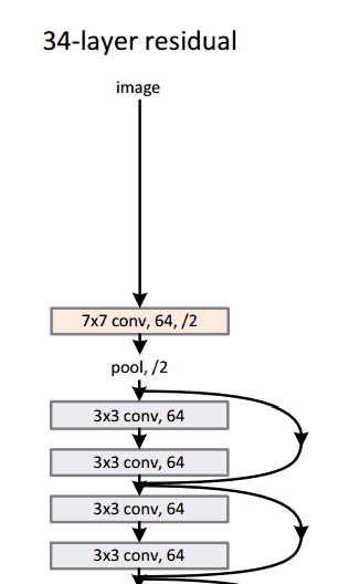
Microsoft ResNet (2015)
Imagine a deep CNN architecture. Take that, double the number of layers, add a couple more, and it still probably isn’t as deep as the ResNet architecture that Microsoft Research Asia came up with in late 2015. ResNet is a new 152 layer network architecture that set new records in classification, detection, and localization through one incredible architecture. Aside from the new record in terms of number of layers, ResNet won ILSVRC 2015 with an incredible error rate of 3.6% (Depending on their skill and expertise, humans generally hover around a 5-10% error rate. See Andrej Karpathy’s great post on his experiences with competing against ConvNets on the ImageNet challenge).
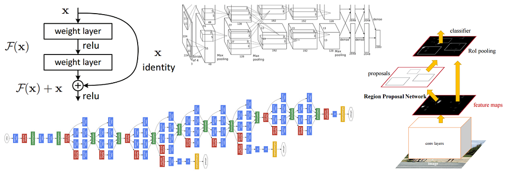
Residual Block
The idea behind a residual block is that you have your input x go through conv-relu-conv series. This will give you some F(x). That result is then added to the original input x. Let’s call that H(x) = F(x) + x. In traditional CNNs, your H(x) would just be equal to F(x) right? So, instead of just computing that transformation (straight from x to F(x)), we’re computing the term that you have to add, F(x), to your input, x. Basically, the mini module shown below is computing a “delta” or a slight change to the original input x to get a slightly altered representation (When we think of traditional CNNs, we go from x to F(x) which is a completely new representation that doesn’t keep any information about the original x). The authors believe that “it is easier to optimize the residual mapping than to optimize the original, unreferenced mapping”.
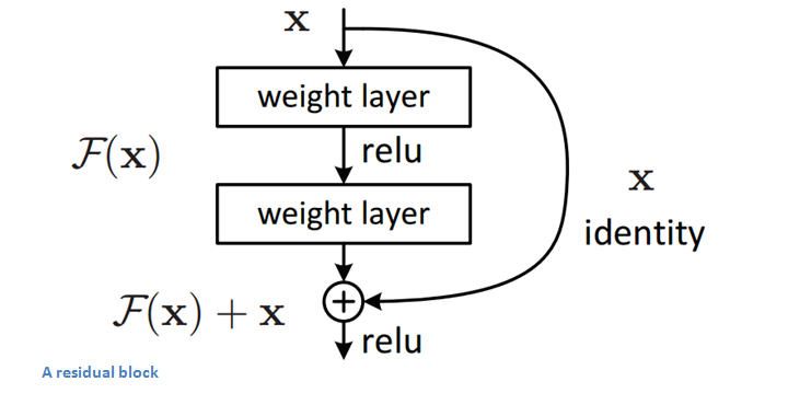
Another reason for why this residual block might be effective is that during the backward pass of backpropagation, the gradient will flow easily through the effective because we have addition operations, which distributes the gradient.
Main Points
- “Ultra-deep” – Yann LeCun.
- 152 layers…
- Interesting note that after only the first 2 layers, the spatial size gets compressed from an input volume of 224x224 to a 56x56 volume.
- Authors claim that a naïve increase of layers in plain nets result in higher training and test error (Figure 1 in the paper).
- The group tried a 1202-layer network, but got a lower test accuracy, presumably due to overfitting.
- Trained on an 8 GPU machine for two to three weeks.
Why It’s Important
3.6% error rate. That itself should be enough to convince you. The ResNet model is the best CNN architecture that we currently have and is a great innovation for the idea of residual learning. With error rates dropping every year since 2012, I’m skeptical about whether or not they will go down for ILSVRC 2016. I believe we’ve gotten to the point where stacking more layers on top of each other isn’t going to result in a substantial performance boost. There would definitely have to be creative new architectures like we’ve seen the last 2 years. On September 16th, the results for this year’s competition will be released. Mark your calendar.
Bonus: ResNets inside of ResNets. Yeah. I went there.
Region Based CNNs (R-CNN - 2013, Fast R-CNN - 2015, Faster R-CNN - 2015)
Some may argue that the advent of R-CNNs has been more impactful that any of the previous papers on new network architectures. With the first R-CNN paper being cited over 1600 times, Ross Girshick and his group at UC Berkeley created one of the most impactful advancements in computer vision. As evident by their titles, Fast R-CNN and Faster R-CNN worked to make the model faster and better suited for modern object detection tasks.
The purpose of R-CNNs is to solve the problem of object detection. Given a certain image, we want to be able to draw bounding boxes over all of the objects. The process can be split into two general components, the region proposal step and the classification step.
The authors note that any class agnostic region proposal method should fit. Selective Search is used in particular for RCNN. Selective Search performs the function of generating 2000 different regions that have the highest probability of containing an object. After we’ve come up with a set of region proposals, these proposals are then “warped” into an image size that can be fed into a trained CNN (AlexNet in this case) that extracts a feature vector for each region. This vector is then used as the input to a set of linear SVMs that are trained for each class and output a classification. The vector also gets fed into a bounding box regressor to obtain the most accurate coordinates.
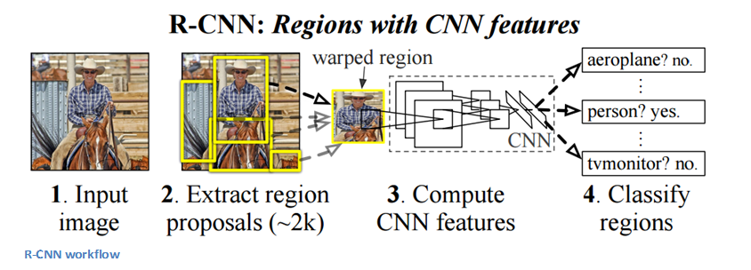
Non-maxima suppression is then used to suppress bounding boxes that have a significant overlap with each other.
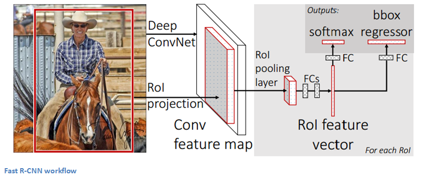
Fast R-CNN
Improvements were made to the original model because of 3 main problems. Training took multiple stages (ConvNets to SVMs to bounding box regressors), was computationally expensive, and was extremely slow (RCNN took 53 seconds per image). Fast R-CNN was able to solve the problem of speed by basically sharing computation of the conv layers between different proposals and swapping the order of generating region proposals and running the CNN. In this model, the image is firstfed through a ConvNet, features of the region proposals are obtained from the last feature map of the ConvNet (check section 2.1 of the paper for more details), and lastly we have our fully connected layers as well as our regression and classification heads.
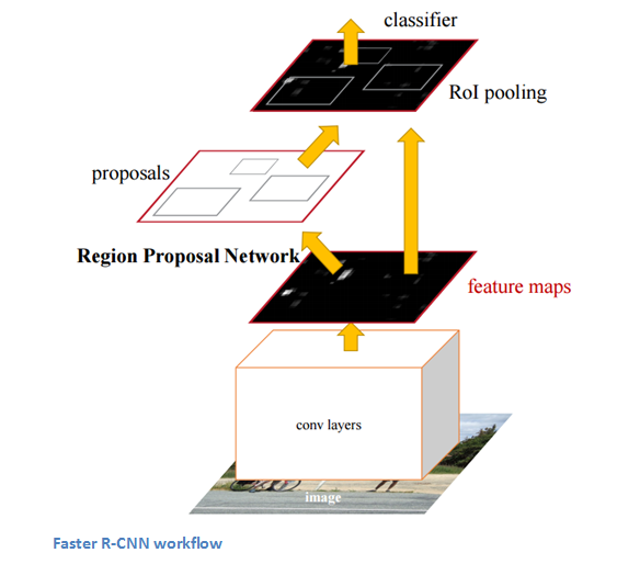
Faster R-CNN
Faster R-CNN works to combat the somewhat complex training pipeline that both R-CNN and Fast R-CNN exhibited. The authors insert a region proposal network (RPN) after the last convolutional layer. This network is able to just look at the last convolutional feature map and produce region proposals from that. From that stage, the same pipeline as R-CNN is used (ROI pooling, FC, and then classification and regression heads).
Why It’s Important
Being able to determine that a specific object is in an image is one thing, but being able to determine that object’s exact location is a huge jump in knowledge for the computer. Faster R-CNN has become the standard for object detection programs today.
Generative Adversarial Networks (2014)
According to Yann LeCun, these networks could be the next big development. Before talking about this paper, let’s talk a little about adversarial examples. For example, let’s consider a trained CNN that works well on ImageNet data. Let’s take an example image and apply a perturbation, or a slight modification, so that the prediction error is maximized. Thus, the object category of the prediction changes, while the image itself looks the same when compared to the image without the perturbation. From the highest level, adversarial examples are basically the images that fool ConvNets.
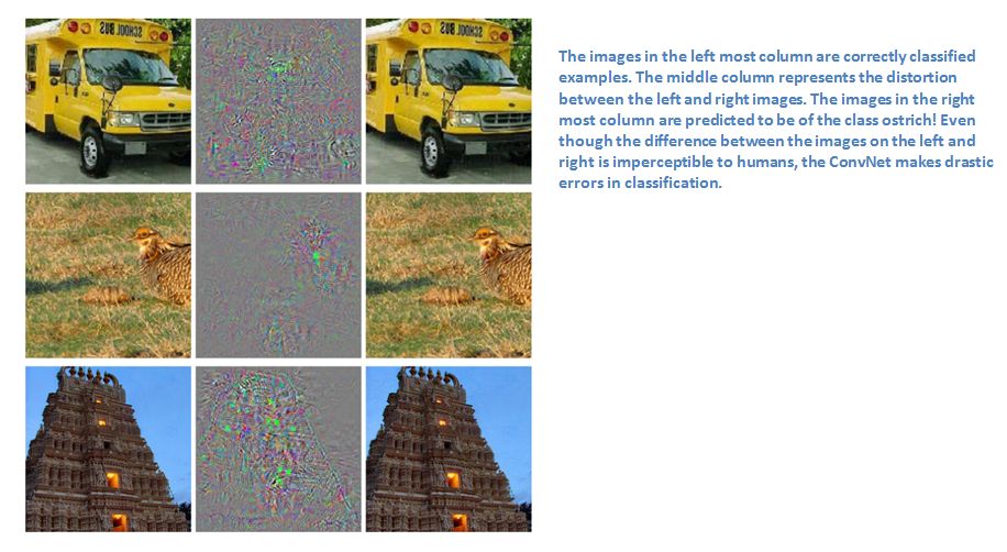
Adversarial examples (paper) definitely surprised a lot of researchers and quickly became a topic of interest. Now let’s talk about the generative adversarial networks. Let’s think of two models, a generative model and a discriminative model. The discriminative model has the task of determining whether a given image looks natural (an image from the dataset) or looks like it has been artificially created. The task of the generator is to create images so that the discriminator gets trained to produce the correct outputs. This can be thought of as a zero-sum or minimax two player game. The analogy used in the paper is that the generative model is like “a team of counterfeiters, trying to produce and use fake currency” while the discriminative model is like “the police, trying to detect the counterfeit currency”. The generator is trying to fool the discriminator while the discriminator is trying to not get fooled by the generator. As the models train, both methods are improved until a point where the “counterfeits are indistinguishable from the genuine articles”.
Why It’s Important
Sounds simple enough, but why do we care about these networks? As Yann LeCun stated in his Quora post, the discriminator now is aware of the “internal representation of the data” because it has been trained to understand the differences between real images from the dataset and artificially created ones. Thus, it can be used as a feature extractor that you can use in a CNN. Plus, you can just create really cool artificial images that look pretty natural to me (link).
Generating Image Descriptions (2014)
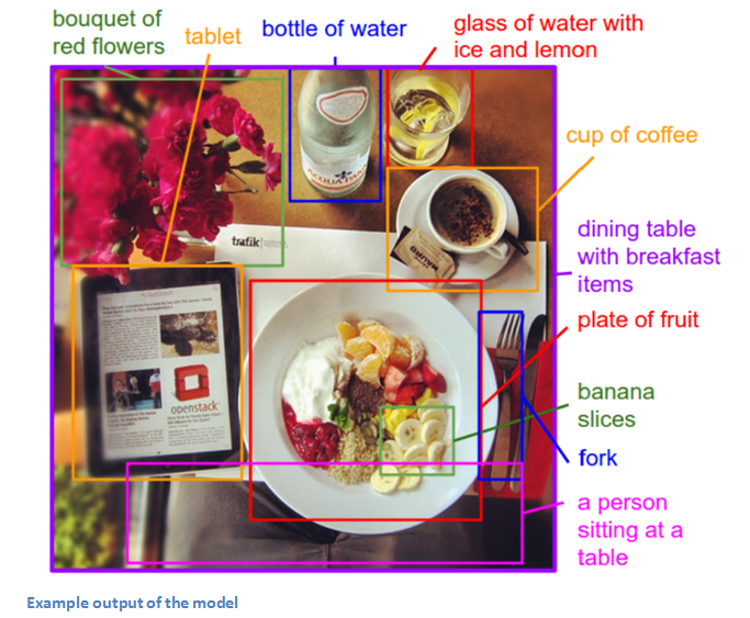
What happens when you combine CNNs with RNNs (No, you don’t get R-CNNs, sorry )?But you do get one really amazing application. Written by Andrej Karpathy (one of my personal favorite authors) and Fei-Fei Li, this paper looks into a combination of CNNs and bidirectional RNNs (Recurrent Neural Networks) to generate natural language descriptions of different image regions. Basically, the model is able to take in an image, and output this:
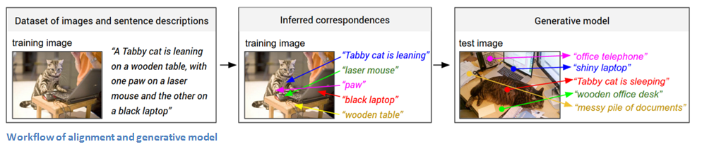
That’s pretty incredible. Let’s look at how this compares to normal CNNs. With traditional CNNs, there is a single clear label associated with each image in the training data. The model described in the paper has training examples that have a sentence (or caption) associated with each image. This type of label is called a weak label, where segments of the sentence refer to (unknown) parts of the image. Using this training data, a deep neural network “infers the latent alignment between segments of the sentences and the region that they describe” (quote from the paper). Another neural net takes in the image as input and generates a description in text. Let’s take a separate look at the two components, alignment and generation.
Alignment Model
The goal of this part of the model is to be able to align the visual and textual data (the image and its sentence description). The model works by accepting an image and a sentence as input, where the output is a score for how well they match (Now, Karpathy refers a different paper which goes into the specifics of how this works. This model is trained on compatible and incompatible image-sentence pairs).
Now let’s think about representing the images. The first step is feeding the image into an R-CNN in order to detect the individual objects. This R-CNN was trained on ImageNet data. The top 19 (plus the original image) object regions are embedded to a 500 dimensional space. Now we have 20 different 500 dimensional vectors (represented by v in the paper) for each image. We have information about the image. Now, we want information about the sentence. We’re going to embed words into this same multimodal space. This is done by using a bidirectional recurrent neural network. From the highest level, this serves to illustrate information about the context of words in a given sentence. Since this information about the picture and the sentence are both in the same space, we can compute inner products to show a measure of similarity.
Generation Model
The alignment model has the main purpose of creating a dataset where you have a set of image regions (found by the RCNN) and corresponding text (thanks to the BRNN). Now, the generation model is going to learn from that dataset in order to generate descriptions given an image. The model takes in an image and feeds it through a CNN. The softmax layer is disregarded as the outputs of the fully connected layer become the inputs to another RNN. For those that aren’t as familiar with RNNs, their function is to basically form probability distributions on the different words in a sentence (RNNs also need to be trained just like CNNs do).
Disclaimer: This was definitely one of the more dense papers in this section, so if anyone has any corrections or other explanations, I’d love to hear them in the comments!
Why It’s Important
The interesting idea for me was that of using these seemingly different RNN and CNN models to create a very useful application that in a way combines the fields of Computer Vision and Natural Language Processing. It opens the door for new ideas in terms of how to make computers and models smarter when dealing with tasks that cross different fields.
Spatial Transformer Networks (2015)
Last, but not least, let’s get into one of the more recent papers in the field. This paper was written by a group at Google Deepmind a little over a year ago. The main contribution is the introduction of a Spatial Transformer module. The basic idea is that this module transforms the input image in a way so that the subsequent layers have an easier time making a classification. Instead of making changes to the main CNN architecture itself, the authors worry about making changes to the image before it is fed into the specific conv layer. The 2 things that this module hopes to correct are pose normalization (scenarios where the object is tilted or scaled) and spatial attention (bringing attention to the correct object in a crowded image). For traditional CNNs, if you wanted to make your model invariant to images with different scales and rotations, you’d need a lot of training examples for the model to learn properly. Let’s get into the specifics of how this transformer module helps combat that problem.
The entity in traditional CNN models that dealt with spatial invariance was the maxpooling layer. The intuitive reasoning behind this later was that once we know that a specific feature is in the original input volume (wherever there are high activation values), it’s exact location is not as important as its relative location to other features. This new spatial transformer is dynamic in a way that it will produce different behavior (different distortions/transformations) for each input image. It’s not just as simple and pre-defined as a traditional maxpool. Let’s take look at how this transformer module works. The module consists of:
- A localization network which takes in the input volume and outputs parameters of the spatial transformation that should be applied. The parameters, or theta, can be 6 dimensional for an affine transformation.
- The creation of a sampling grid that is the result of warping the regular grid with the affine transformation (theta) created in the localization network.
- A sampler whose purpose is to perform a warping of the input feature map.
This module can be dropped into a CNN at any point and basically helps the network learn how to transform feature maps in a way that minimizes the cost function during training.
Why It’s Important
This paper caught my eye for the main reason that improvements in CNNs don’t necessarily have to come from drastic changes in network architecture. We don’t need to create the next ResNet or Inception module. This paper implements the simple idea of making affine transformations to the input image in order to help models become more invariant to translation, scale, and rotation. For those interested, here is a video from Deepmind that has a great animation of the results of placing a Spatial Transformer module in a CNN and a good Quora discussion.
And that ends our 3 part series on ConvNets! Hope everyone was able to follow along, and if you feel that I may have left something important out, let me know in the comments! If you want more info on some of these concepts, I once again highly recommend Stanford CS 231n lecture videos which can be found with a simple YouTube search.
Dueces.
Sources