Zero-shot Recognition via semantic embeddings and knowledege graphs
2018-03-31 15:38:39
【Abstract】
我们考虑 zero-shot recognition 的问题:学习一个类别的视觉分类器,并且不用 training data,仅仅依赖于 类别的单词映射(the word embedding of the category)及其与其他类别的关系(its relationship to other categories),但是会提供 visual data。处理这种不熟悉的或者新颖的类别,从已有的类别中进行知识的迁移是成功的关键。本文,我们通过引入 GCN,然后提出一种方法同时利用 semantic embeddings 以及 categorical knowledge graph 来预测分类器。给定一个学习的知识图谱(a learned knowledge graph (KG)),我们的方法将 semantic embeddings for each node (representing visual category)。在一系列的 graph convolutions 之后,我们对每一个种类预测 the visual predictor。在训练的过程中,一些类别的 visual classifiers 是给定的,用来学习 the GCN parameters。在测试的时候,这些 filters 被用来预测未见种类的 visual classifiers。
【Introduction】
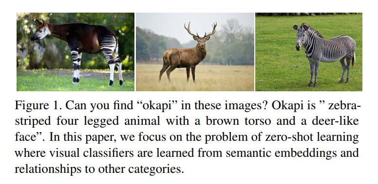
现有的物体分类的方法,都需要大量的训练数据,然后针对每一类训练一个分类器。但是,当新增加一个类别的时候,又需要再训练一个 model,并且还需要收集大量的数据。为了解决这个问题,zero-shot learning 经常被用到。处理 unfamiliar 或者 novel category 的关键是:从熟悉的种类进行知识的迁移,来描述不熟悉的类别(generalization)。
有两种迁移知识的方法。
第一种是利用 implicit knowledge representation,即:semantic embeddings。在这种方法中,one learns a vector representation of different categories using text data and then learns a mapping between the vector representation to visual classifier directly. 但是,这些方法受限于 the generalization power of the semantic models and the mapping models themselves. It is also hard to learn semantic embeddings from structured information.
另一种进行 zero-shot learning 的方法是:利用现有的知识库或者知识图谱(explicit knowledge bases or knowledge graphs)。在这个流程中,我们显示的将知识图谱表达为:rules or relationships between objects。这些关系可以进行 new categories 的 zero-shot classifiers 的学习。一个很有意思的问题是,我们想要探讨:if we can use structured information and complex relationships to learn visual classifiers without seeing any examples。
在本文当中,我们提出提取 隐式的知识表示(the implicit knowledge representation,i.e. Word embedding)以及 显示的表示(the explicit relationships, i.e. knowledge graph)来学习新颖种类的视觉分类器(for learning visual classifiers of novel classes)。我们构建一个知识图谱,每一个节点代表了一个 semantic category。这些节点用 relationship edges 来进行连接。该graph 节点的输入是:每一个种类的向量表示(the vector representation of each category)。我们然后用 Graph Convolutional Network(GCN)来进行不同种类之间的信息迁移(transfer information between different catrgories)。特别的,我们训练一个 6-layer deep GCN 来输出不同种类的类别(that outputs the classifiers of different categories)。
我们集中于 image classification,我们考虑两种测试的设置:
(a)final test classes being only zero-shot classes (without training classes at test time) ;
(b)at test time the labels can be either the seen or the unseen classes, namely "generalized zero-shot learning"。
跟传统方法对比,我们取得了令人惊奇的好结果,that is a whopping 18.7% improvement over the current state-of-the-art。
【Approach】
我们的目标是从显示的和隐式的表达中进行信息提取,然后进行 zero-shot classification。我们在 GCN 的基础上学习 visual classifiers。我们首先介绍 如何将 GCN 引入 NLP 领域进行分类任务,然后将详细讨论:applying the GCN with a regression loss for zero-shot learning。
3.1. Background: Graph Convolutional Network
GCN 被引入执行 semi-supervised entity classfication. 给定 object entities,用 Word embeddings or text features, 任务是进行分类。例如:将“dog” and "cat" 分类为 “mammal”;“chair” 以及 “couch”分类为“furniture”。我们也假设有这么一个 graph,其节点代表的是 entities。边代表的是 entities 之间的关系。
正式的,给定一个数据集,有 n 个 entities (X, Y)= ${(xi, yi)}_{i=1}^n$,其中,xi 代表的是 entities i 的 Word embedding,yi 代表其 label。在半监督的设定下,我们知道 semi-supervised setting下,我们知道前 m 个 entities 的 ground truth labels。我们的目标是利用 Word embedding 以及 the relationships graph,去推断 the remaining n-m entities,而这些是没有标签的。
我们用函数 F(*) 来表示 GCN。其将所有的映射后的 X 作为输入,然后输出所有的 softmax classification results F(X)。简单起见,我们表示 第 i 个 entity 的输出为 Fi(X),是一个 C维的 softmax probability vector。在训练的时候,我们采用 softmax loss 进行训练:
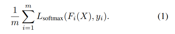
F(*) 的权重是利用该 loss 通过反向传播算法进行训练的。在测试的时候,我们利用学习到的权重来获得剩下 n-m entities 的 label。
不像在图像上局部区域进行卷积操作一样,在 GCN 中,the convolutional operations 计算一个节点的相应,是基于定义在 the adjacency matrix 上的紧邻节点的(compute the response at a node based on the neighboring nodes defined by the adjacency graph)。数学上来讲,在 Graph 上进行网络 F(*) 每一层的卷积操作可以表达为:
![]()
其中,$A^{^}$是 graph 的二元紧邻矩阵A 的归一化版本(the normalized version of the binary adjacency matrix A of the graph),其维度为:n*n dimension。X' 是来自上一层的 n*k feature matrix。W是 the weigth matrix of the layer with dimension k*c,其中,c 是输出通道个数。所以,卷积层的输入是 n*k,输出是 n*c matrix Z。这些卷积操作可以一层一层的累积。在每一层之后,用 ReLU 进行非线性处理。对于最后的 convolutional layer,输出通道的 channel 是 label classes (c = C)。
3.2. GCN for Zero-shot Learning :
我们的模型是在 GCN 的基础上构建起来的,然而,不像是 entity classification,我们用一个 regression loss 来应用于 zero-shot recognition。我们框架的输入是:the set of categories and their corresponding semantic-embedding vectors。输出是:the visual classifier for each input category。
特别的,我们想用 GCN 去学习的 visual classifier 是:a logistic regression model on the fixed pre-trained ConvNet features. 如果 visual-feature 的维度是D,那么,每一个 classifier $w_i$ 也是 D-dimensional vector。所以,GCN 中每一个节点的输出是 D 维,而不是 C 维。在 zero-shot learning 中,我们假设总共 n 类的 first m categories 拥有足够的 visual examples 来预测他们的权重向量。对于剩下的 n-m种,输入他们的 embedding vectors,我们想要预测他们各自的权重向量。
一种训练 neural network(multi-layer perceptron)的方法是:将 xi 作为输入,然后学习预测 wi 作为输出。网络的参数可以用 m 对训练样本进行预测。然而,总体上来说,m 总是小的(in the order of a few hundreds),我们想要显示的利用 visual world 的结构,或者种类之间的关系来约束该问题。我们用知识图谱(knowledge graph)来表示他们的关系。每一个节点代表了一个 semantic category。因为我们总共有 n 个种类,在 graph 中有 n 个节点。如果两个节点之间存在某种关系,就将其连接起来。图结构表示为 n*n 的邻接矩阵,A。在本文中,我们用 undirected edges 代替 KG 中所有的 directed edges,这样就得到了一个对称的 adjacency matrix。
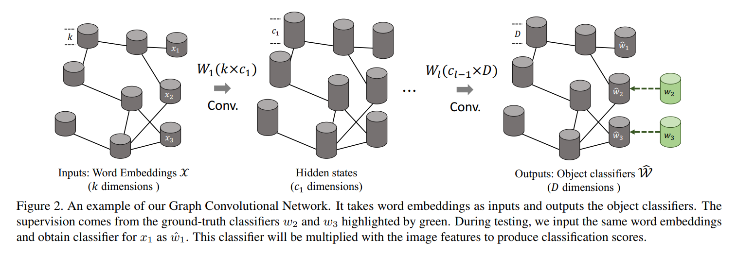
像图2中所示,我们用一个 6-layer GCN,每一层输入是 feature representation,输出是一个新的 feature representation。对于第一层,输入 X 是一个 n*k matrix ( k is the dimensionaltiy of the word-embedding vector)。对于最后一层,输出的 feature vector W^,其维度为:n*D;D 是分类器或者视觉向量的维度。
Loss-function:对于前 m 个类别,我们预测分类器的权重 $hat{W}_{1, 2, ... , m}$ ,从训练数据中学习的 GT classifier weights。此处利用 MSE 来训练:
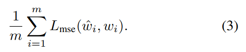
在训练的过程中,我们利用 m 个可见的类别得到的 loss 来预测 GCN 的参数。利用预测的参数,我们得到 the zero-shot categories 的分类器权重。在测试的时候,我们利用 pre-trained convnet 来提取 image feature representation,然后利用这些产生的分类器来进行图像的分类。
3.3. Implementation Details :
我们的 GCN 由 6 个 convolutional layers 构成,输出的 channel 分别为:2048->2048->1024->1024->512->D,其中 D 代表了物体分类器的维度。当训练我们的 GCN 时,我们在网络的输出以及 GT classifier 上,执行 L2-Normalization。在测试的过程中,the unseen classes 产生的分类器也是 L2-Normalized。我们发现,添加该重要的约束,as it regularizes the weights of all the classifiers into similar magnitudes。
为了得到 GCN 输入的 Word embeddings,我们利用 GloVe text model 在 Wikipedia dataset,which leads to 300-d vectors. 对于类别包含多个单词的名字,我们在训练模型上匹配所有的单词,然后找到他们的映射。通过平均这些单词映射,我们得到其类别映射(by averaging these word embeddings, we obtain the class embedding)。
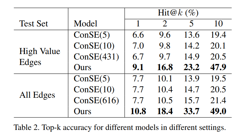
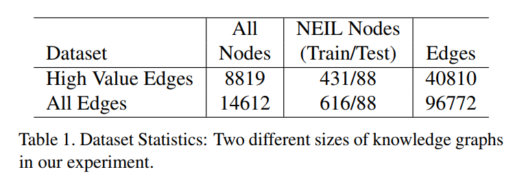
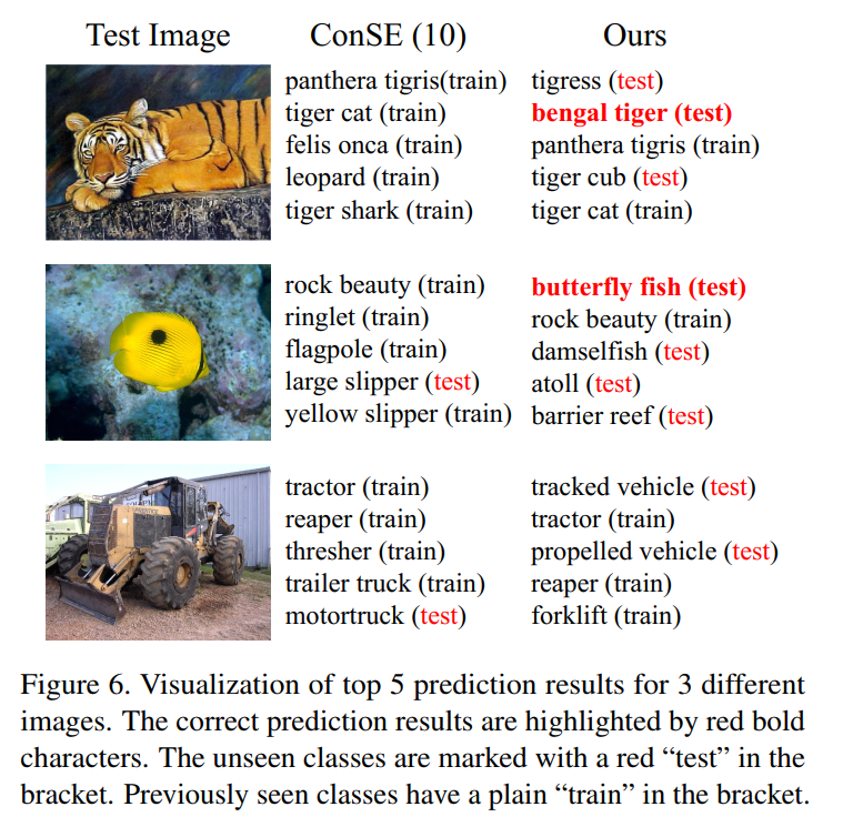
【Experiments】