实验一

一、环境

pycharm tensorflow1.15 python3.7 sklearn

二、波士顿房价预测实验

from sklearn.linear_model import LinearRegression, SGDRegressor, Ridge, LogisticRegression
from sklearn.datasets import load_boston
from sklearn.model_selection import train_test_split
from sklearn.preprocessing import StandardScaler
from sklearn.metrics import mean_squared_error
#from sklearn.externals import joblib
from sklearn.metrics import r2_score
from sklearn.neural_network import MLPRegressor

import pandas as pd
import numpy as np

lb = load_boston()
x_train, x_test, y_train, y_test = train_test_split(lb.data, lb.target, test_size=0.2)


# 为数据增加一个维度,相当于把[1, 5, 10] 变成 [[1, 5, 10],]
y_train = y_train.reshape(-1, 1)#列数为1
y_test = y_test.reshape(-1, 1)

# 进行标准化
std_x = StandardScaler()#标准化数据
x_train = std_x.fit_transform(x_train)#对数据进行某种统一处理
x_test = std_x.transform(x_test)

std_y = StandardScaler()
y_train = std_y.fit_transform(y_train)
y_test = std_y.transform(y_test)
# 正规方程预测
lr = LinearRegression()#线性回归
lr.fit(x_train, y_train)
print("r2 score of Linear regression is",r2_score(y_test,lr.predict(x_test)))
#岭回归
from sklearn.linear_model import RidgeCV

cv = RidgeCV(alphas=np.logspace(-3, 2, 100))#样本数据集
cv.fit (x_train , y_train)
print("r2 score of Linear regression is",r2_score(y_test,cv.predict(x_test)))
#梯度下降
sgd = SGDRegressor()#最大迭代次数
sgd.fit(x_train, y_train)#用训练器数据拟合分类器模型
print("r2 score of Linear regression is",r2_score(y_test,sgd.predict(x_test)))

三、鸢尾花分类

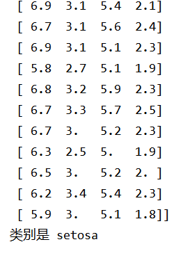
from sklearn import datasets
import matplotlib.pyplot as plt
import numpy as np
from sklearn import tree

# Iris数据集是常用的分类实验数据集，
# 由Fisher, 1936收集整理。Iris也称鸢尾花卉数据集，
# 是一类多重变量分析的数据集。数据集包含150个数据集，
# 分为3类，每类50个数据，每个数据包含4个属性。
# 可通过花萼长度，花萼宽度，花瓣长度，花瓣宽度4个属性预测鸢尾花卉属于（Setosa，Versicolour，Virginica）三个种类中的哪一类。

# 载入数据集
iris = datasets.load_iris()#数据集
iris_data = iris['data']
iris_label = iris['target']
iris_target_name = iris['target_names']
X = np.array(iris_data)
Y = np.array(iris_label)
print(X)
# 训练
clf = tree.DecisionTreeClassifier(max_depth=3)
clf.fit(X, Y)

# 这里预测当前输入的值的所属分类
print('类别是', iris_target_name[clf.predict([[12, 1, -1, 10]])[0]])

实验截图：

四、特征处理（标准化、归一化、正则化）

4.1

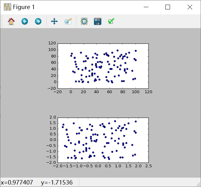
from sklearn.preprocessing import StandardScaler
from sklearn.preprocessing import MinMaxScaler
from matplotlib import gridspec
import numpy as np
import matplotlib.pyplot as plt

cps = np.random.random_integers(0, 100, (100, 2))

ss = StandardScaler()#标准化归一化
std_cps = ss.fit_transform(cps)#对数据进行某种统一处理

gs = gridspec.GridSpec(5, 5)#创建区域，参数5，5的意思就是每行五个，每列五个，最后就是一个5×5的画布
fig = plt.figure()#创建画布
ax1 = fig.add_subplot(gs[0:2, 1:4])#在画布上创建不同的区域
ax2 = fig.add_subplot(gs[3:5, 1:4])

ax1.scatter(cps[:, 0], cps[:, 1])#标准化
ax2.scatter(std_cps[:, 0], std_cps[:, 1])

plt.show()

实验截图：

4.2

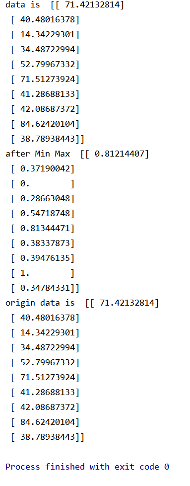
from sklearn.preprocessing import MinMaxScaler
import numpy as np

data = np.random.uniform(0, 100, 10)[:, np.newaxis]#从零位对浮点数组做舍入
mm = MinMaxScaler()#归一化特征到一定区间
mm_data = mm.fit_transform(data)#对数据进行某种统一处理
origin_data = mm.inverse_transform(mm_data)#将标准化后的数据转换为原始数据。
print('data is ',data)
print('after Min Max ',mm_data)
print('origin data is ',origin_data)

实验截图：

4.3

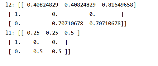
X = [[1, -1, 2],
     [2, 0, 0],
     [0, 1, -1]]

# 使用L2正则化
from sklearn.preprocessing import normalize
l2 = normalize(X, norm='l2')#数据预处理
print('l2:', l2)

# 使用L1正则化
from sklearn.preprocessing import Normalizer
normalizerl1 = Normalizer(norm='l1')#对每个样本的每一个元素都除以该样本的L1范数. 
l1 = normalizerl1.fit_transform(X)
print('l1:', l1)

实验截图：

 五、交叉验证

from sklearn.model_selection import train_test_split,cross_val_score,cross_validate # 交叉验证所需的函数
from sklearn.model_selection import KFold,LeaveOneOut,LeavePOut,ShuffleSplit # 交叉验证所需的子集划分方法
from sklearn.model_selection import StratifiedKFold,StratifiedShuffleSplit # 分层分割
from sklearn.model_selection import GroupKFold,LeaveOneGroupOut,LeavePGroupsOut,GroupShuffleSplit # 分组分割
from sklearn.model_selection import TimeSeriesSplit # 时间序列分割
from sklearn import datasets  # 自带数据集
from sklearn import svm  # SVM算法
from sklearn import preprocessing  # 预处理模块
from sklearn.metrics import recall_score  # 模型度量

iris = datasets.load_iris()  # 加载数据集
print('样本集大小：',iris.data.shape,iris.target.shape)

# ===================================数据集划分,训练模型==========================
X_train, X_test, y_train, y_test = train_test_split(iris.data, iris.target, test_size=0.4, random_state=0)  # 交叉验证划分训练集和测试集.test_size为测试集所占的比例
print('训练集大小：',X_train.shape,y_train.shape)  # 训练集样本大小
print('测试集大小：',X_test.shape,y_test.shape)  # 测试集样本大小
clf = svm.SVC(kernel='linear', C=1).fit(X_train, y_train) # 使用训练集训练模型
print('准确率：',clf.score(X_test, y_test))  # 计算测试集的度量值（准确率）


#  如果涉及到归一化，则在测试集上也要使用训练集模型提取的归一化函数。
scaler = preprocessing.StandardScaler().fit(X_train)  # 通过训练集获得归一化函数模型。（也就是先减几，再除以几的函数）。在训练集和测试集上都使用这个归一化函数
X_train_transformed = scaler.transform(X_train)
clf = svm.SVC(kernel='linear', C=1).fit(X_train_transformed, y_train) # 使用训练集训练模型
X_test_transformed = scaler.transform(X_test)
print(clf.score(X_test_transformed, y_test))  # 计算测试集的度量值（准确度）

# ===================================直接调用交叉验证评估模型==========================
clf = svm.SVC(kernel='linear', C=1)
scores = cross_val_score(clf, iris.data, iris.target, cv=5)  #cv为迭代次数。
print(scores)  # 打印输出每次迭代的度量值（准确度）
print("Accuracy: %0.2f (+/- %0.2f)" % (scores.mean(), scores.std() * 2))  # 获取置信区间。（也就是均值和方差）

# ===================================多种度量结果======================================
scoring = ['precision_macro', 'recall_macro'] # precision_macro为精度，recall_macro为召回率
scores = cross_validate(clf, iris.data, iris.target, scoring=scoring,cv=5, return_train_score=True)
sorted(scores.keys())
print('测试结果：',scores)  # scores类型为字典。包含训练得分，拟合次数， score-times （得分次数）


# ==================================K折交叉验证、留一交叉验证、留p交叉验证、随机排列交叉验证==========================================
# k折划分子集
kf = KFold(n_splits=2)
for train, test in kf.split(iris.data):
    print("k折划分：%s %s" % (train.shape, test.shape))
    break

# 留一划分子集
loo = LeaveOneOut()
for train, test in loo.split(iris.data):
    print("留一划分：%s %s" % (train.shape, test.shape))
    break

# 留p划分子集
lpo = LeavePOut(p=2)
for train, test in loo.split(iris.data):
    print("留p划分：%s %s" % (train.shape, test.shape))
    break

# 随机排列划分子集
ss = ShuffleSplit(n_splits=3, test_size=0.25,random_state=0)
for train_index, test_index in ss.split(iris.data):
    print("随机排列划分：%s %s" % (train.shape, test.shape))
    break

# ==================================分层K折交叉验证、分层随机交叉验证==========================================
skf = StratifiedKFold(n_splits=3)  #各个类别的比例大致和完整数据集中相同
for train, test in skf.split(iris.data, iris.target):
    print("分层K折划分：%s %s" % (train.shape, test.shape))
    break

skf = StratifiedShuffleSplit(n_splits=3)  # 划分中每个类的比例和完整数据集中的相同
for train, test in skf.split(iris.data, iris.target):
    print("分层随机划分：%s %s" % (train.shape, test.shape))
    break


# ==================================组 k-fold交叉验证、留一组交叉验证、留 P 组交叉验证、Group Shuffle Split==========================================
X = [0.1, 0.2, 2.2, 2.4, 2.3, 4.55, 5.8, 8.8, 9, 10]
y = ["a", "b", "b", "b", "c", "c", "c", "d", "d", "d"]
groups = [1, 1, 1, 2, 2, 2, 3, 3, 3, 3]

# k折分组
gkf = GroupKFold(n_splits=3)  # 训练集和测试集属于不同的组
for train, test in gkf.split(X, y, groups=groups):
    print("组 k-fold分割：%s %s" % (train, test))

# 留一分组
logo = LeaveOneGroupOut()
for train, test in logo.split(X, y, groups=groups):
    print("留一组分割：%s %s" % (train, test))

# 留p分组
lpgo = LeavePGroupsOut(n_groups=2)
for train, test in lpgo.split(X, y, groups=groups):
    print("留 P 组分割：%s %s" % (train, test))

# 随机分组
gss = GroupShuffleSplit(n_splits=4, test_size=0.5, random_state=0)
for train, test in gss.split(X, y, groups=groups):
    print("随机分割：%s %s" % (train, test))


# ==================================时间序列分割==========================================
tscv = TimeSeriesSplit(n_splits=3)
TimeSeriesSplit(max_train_size=None, n_splits=3)
for train, test in tscv.split(iris.data):
    print("时间序列分割：%s %s" % (train, test))