
一、 前言
之前看到信用标准评分卡模型开发及实现的文章,是标准的评分卡建模流程在R上的实现,非常不错,就想着能不能把开发流程在Python上实验一遍呢,经过一番折腾后,终于在Python上用类似的代码和包实现出来,由于Python和R上函数的差异以及样本抽样的差异,本文的结果与该文有一定的差异,这是意料之中的,也是正常,接下来就介绍建模的流程和代码实现。
|
1
2
3
4
5
6
7
8
9
10
|
#####代码中需要引用的包#####
import numpy as np
import pandas as pd
from sklearn.utils import shuffle
from sklearn.feature_selection import RFE, f_regression
import scipy.stats.stats as stats
import matplotlib.pyplot as plt
from sklearn.linear_model import LogisticRegression
import math
import matplotlib.pyplot as plt
|
二、数据集准备
数据来自互联网上经常被用来研究信用风险评级模型的加州大学机器学习数据库中的german credit data,原本是存在R包”klaR”中的GermanCredit,我在R中把它加载进去,然后导出csv,最终导入Python作为数据集
|
1
2
3
4
|
############## R #################
library(klaR)
data(GermanCredit ,package="klaR")
write.csv(GermanCredit,"/filePath/GermanCredit.csv")
|
该数据集包含了1000个样本,每个样本包括了21个变量(属性),其中包括1个违约状态变量“credit_risk”,剩余20个变量包括了所有的7个定量和13个定性指标
|
1
2
3
4
5
6
7
8
9
10
11
12
13
14
15
16
17
18
19
20
21
22
23
24
|
>>> df_raw = pd.read_csv('/filePath/GermanCredit.csv')
>>> df_raw.dtypes
Unnamed: 0 int64
status object
duration int64
credit_history object
purpose object
amount int64
savings object
employment_duration object
installment_rate int64
personal_status_sex object
other_debtors object
present_residence int64
property object
age int64
other_installment_plans object
housing object
number_credits int64
job object
people_liable int64
telephone object
foreign_worker object
credit_risk object
|
接下来对数据集进行拆分,按照7:3拆分训练集和测试集,并将违约样本用“1”表示,正常样本用“0”表示。
|
1
2
3
4
5
6
7
8
9
10
11
12
13
14
15
16
17
|
#提取样本训练集和测试集
def split_data(data, ratio=0.7, seed=None):
if seed:
shuffle_data = shuffle(data, random_state=seed)
else:
shuffle_data = shuffle(data, random_state=np.random.randint(10000))
train = shuffle_data.iloc[:int(ratio*len(shuffle_data)), ]
test = shuffle_data.iloc[int(ratio*len(shuffle_data)):, ]
return train, test
#设置seed是为了保证下次拆分的结果一致
df_train,df_test = split_data(df_raw, ratio=0.7, seed=666)
#将违约样本用“1”表示,正常样本用“0”表示。
credit_risk = [0 if x=='good' else 1 for x in df_train['credit_risk']]
#credit_risk = np.where(df_train['credit_risk'] == 'good',0,1)
data = df_train
data['credit_risk']=credit_risk
|
三、定量和定性指标筛选
Python里面可以根据dtype对指标进行定量或者定性的区分,int64为定量指标,object则为定性指标,定量指标的筛选本文通过Python sklearn包中的f_regression进行单变量指标筛选,根据F检验值和P值来选择入模变量
|
1
2
3
4
|
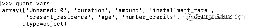
#获取定量指标
quant_index = np.where(data.dtypes=='int64')
quant_vars = np.array(data.columns)[quant_index]
quant_vars = np.delete(quant_vars,0)
|
-
-
|
1
2
3
4
|
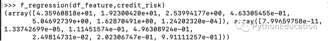
df_feature = pd.DataFrame(data,columns=['duration','amount','installment_rate','present_residence','age','number_credits','people_liable'])
f_regression(df_feature,credit_risk)
#输出逐步回归后得到的变量,选择P值<=0.1的变量
quant_model_vars = ["duration","amount","age","installment_rate"]
|
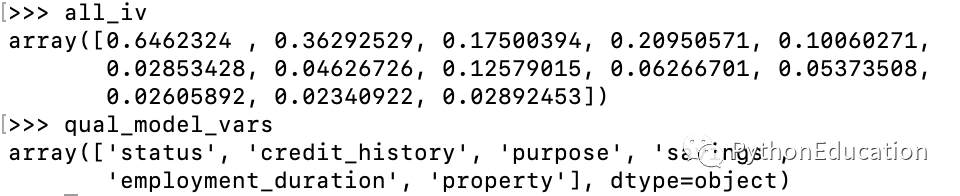
定性指标的筛选可通过计算IV值,并选择IV值大于某一数值的条件来筛选指标,此处自己实现了WOE和IV的函数计算,本文选择了IV值大于0.1的指标,算是比较高的IV值了,一般大于0.02就算是好变量
|
1
2
3
4
5
6
7
8
9
10
11
12
13
14
15
16
|
def woe(bad, good):
return np.log((bad/bad.sum())/(good/good.sum()))
all_iv = np.empty(len(factor_vars))
woe_dict = dict() #存起来后续有用
i = 0
for var in factor_vars:
data_group = data.groupby(var)['credit_risk'].agg([np.sum,len])
bad = data_group['sum']
good = data_group['len']-bad
woe_dict[var] = woe(bad,good)
iv = ((bad/bad.sum()-good/good.sum())*woe(bad,good)).sum()
all_iv[i] = iv
i = i+1
high_index = np.where(all_iv>0.1)
qual_model_vars = factor_vars[high_index]
|
四、连续变量分段和离散变量降维
接下来对连续变量进行分段,由于R包有smbinning自动分箱函数,Python没有,只好采用别的方法进行自动分箱,从网上找了一个monotonic
binning的Python实现,本文进行了改造,增加分段时的排序和woe的计算,还支持手动分箱计算woe,具体代码如下:
|
1
2
3
4
5
6
7
8
9
10
11
12
13
14
15
16
17
18
19
20
21
22
23
24
|
def binning(Y, X, n=None):
# fill missings with median
X2 = X.fillna(np.median(X))
if n == None:
r = 0
n = 10
while np.abs(r) < 1:
#d1 = pd.DataFrame({"X": X2, "Y": Y, "Bucket": pd.qcut(X2, n)})
d1 = pd.DataFrame(
{"X": X2, "Y": Y, "Bucket": pd.qcut(X2.rank(method='first'), n)})
d2 = d1.groupby('Bucket', as_index=True)
r, p = stats.spearmanr(d2.mean().X, d2.mean().Y)
n = n - 1
else:
d1 = pd.DataFrame({"X": X2, "Y": Y, "Bucket": pd.qcut(X2.rank(method='first'), n)})
d2 = d1.groupby('Bucket', as_index=True)
d3 = pd.DataFrame()
d3['min'] = d2.min().X
d3['max'] = d2.max().X
d3['bad'] = d2.sum().Y
d3['total'] = d2.count().Y
d3['bad_rate'] = d2.mean().Y
d3['woe'] = woe(d3['bad'], d3['total'] - d3['bad'])
return d3
|
|
1
2
3
4
5
6
7
8
9
10
11
12
13
14
|
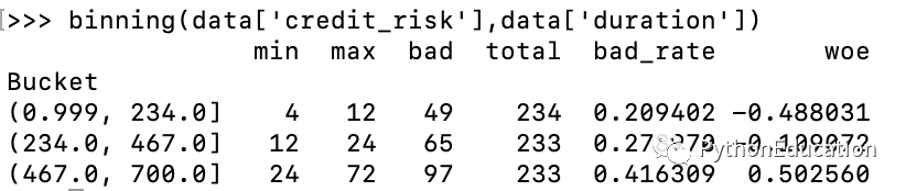
# duration
binning(data['credit_risk'],data['duration'])
duration_Cutpoint=list()
duration_WoE=list()
for x in data['duration']:
if x <= 12:
duration_Cutpoint.append('<= 12')
duration_WoE.append(-0.488031)
if x > 12 and x <= 24:
duration_Cutpoint.append('<= 24')
duration_WoE.append(-0.109072)
if x > 24:
duration_Cutpoint.append('> 24')
duration_WoE.append(0.502560)
|
|
1
2
3
4
5
6
7
8
9
10
11
|
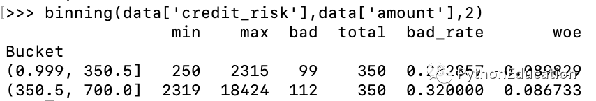
# amount 手动分箱
binning(data['credit_risk'],data['amount'],2)
amount_Cutpoint=list()
amount_WoE=list()
for x in data['amount']:
if x <= 2315:
amount_Cutpoint.append('<= 2315')
amount_WoE.append(-0.089829)
if x > 2315:
amount_Cutpoint.append('> 2315')
amount_WoE.append(0.086733)
|
|
1
2
3
4
5
6
7
8
9
10
11
12
13
14
|
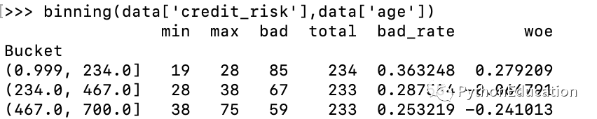
# age
binning(data['credit_risk'],data['age'])
age_Cutpoint=list()
age_WoE=list()
for x in data['age']:
if x <= 28:
age_Cutpoint.append('<= 28')
age_WoE.append(0.279209)
if x > 28 and x <= 38:
age_Cutpoint.append('<= 38')
age_WoE.append(-0.066791)
if x > 38:
age_Cutpoint.append('> 38')
age_WoE.append(-0.241013)
|
|
1
2
3
4
5
6
7
8
9
10
11
12
13
14
|
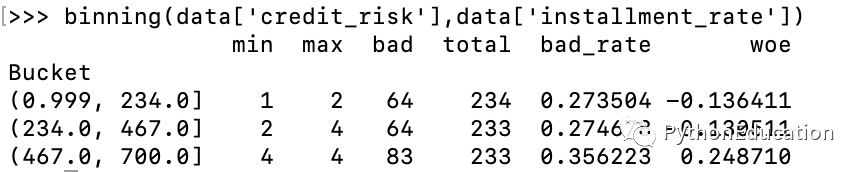
# installment_rate
binning(data['credit_risk'],data['installment_rate'])
nstallment_rate_Cutpoint=list()
installment_rate_WoE=list()
for x in data['installment_rate']:
if x <= 2:
installment_rate_Cutpoint.append('<= 2')
installment_rate_WoE.append(-0.136411)
if x > 2 and x < 4:
installment_rate_Cutpoint.append('< 4')
installment_rate_WoE.append(-0.130511)
if x >= 4:
installment_rate_Cutpoint.append('>= 4')
installment_rate_WoE.append(0.248710)
|
离散变量由于不同变量的维度不一致,为了防止“维数灾难”,对多维对变量进行降维,在评级模型开发中的降维处理方法,通常是将属性相似的合并处理,以达到降维的目的,本文采用参考文献对做法进行合并降维。
|
1
2
3
4
5
6
7
8
9
10
11
12
13
14
15
16
17
18
19
20
21
22
|
#定性指标的降维和WoE
discrete_data = data[qual_model_vars]
discrete_data['credit_risk']= data['credit_risk']
#对purpose指标进行降维
pd.value_counts(data['purpose'])
#合并car(new)、car(used)
discrete_data['purpose'] = discrete_data['purpose'].replace('car (new)', 'car(new/used)')
discrete_data['purpose'] = discrete_data['purpose'].replace('car (used)', 'car(new/used)')
#合并radio/television、furniture/equipment
discrete_data['purpose'] = discrete_data['purpose'].replace('radio/television', 'radio/television/furniture/equipment')
discrete_data['purpose'] = discrete_data['purpose'].replace('furniture/equipment', 'radio/television/furniture/equipment')
#合并others、repairs、business
discrete_data['purpose'] = discrete_data['purpose'].replace('others', 'others/repairs/business')
discrete_data['purpose'] = discrete_data['purpose'].replace('repairs', 'others/repairs/business')
discrete_data['purpose'] = discrete_data['purpose'].replace('business', 'others/repairs/business')
#合并retraining、education
discrete_data['purpose'] = discrete_data['purpose'].replace('retraining', 'retraining/education')
discrete_data['purpose'] = discrete_data['purpose'].replace('education', 'retraining/education')
data_group = discrete_data.groupby('purpose')['credit_risk'].agg([np.sum,len])
bad = data_group['sum']
good = data_group['len']-bad
woe_dict['purpose'] = woe(bad,good)
|
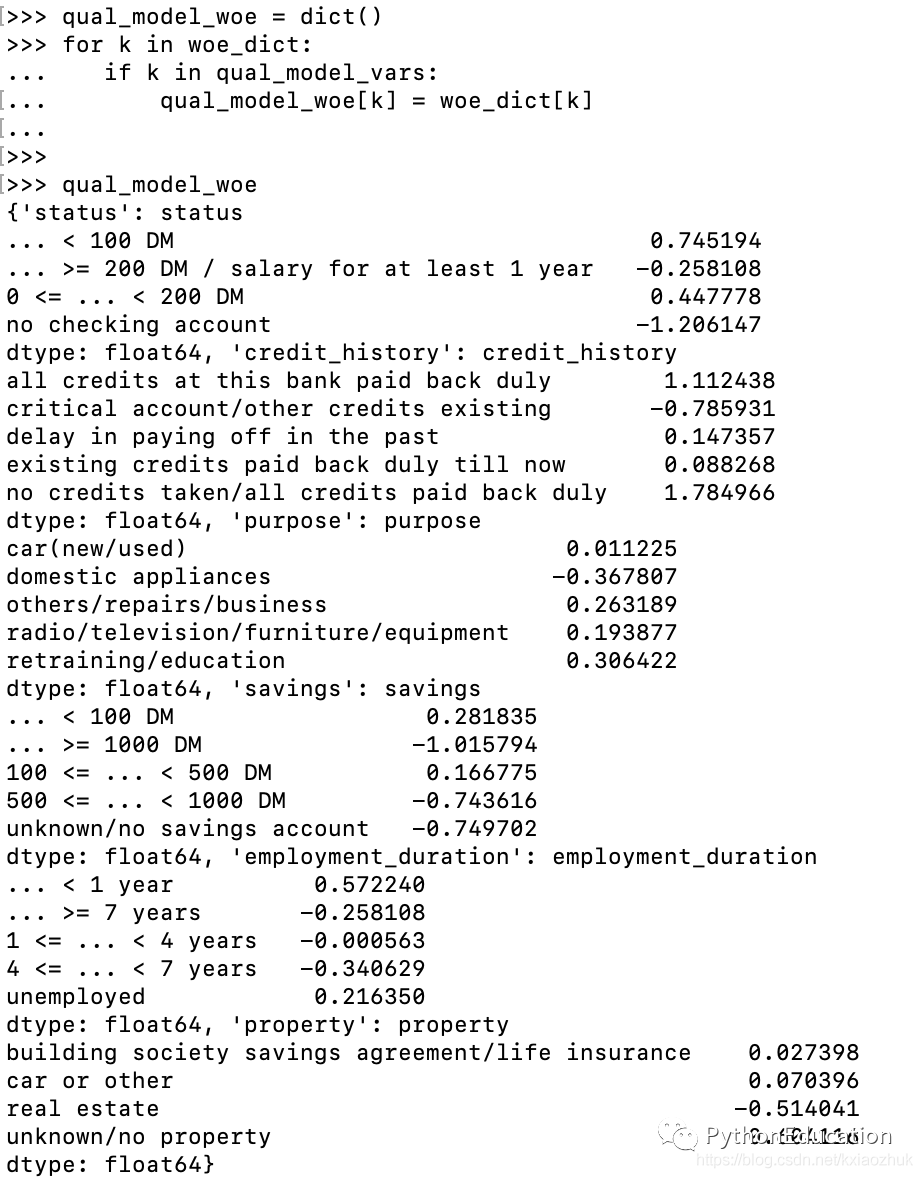
所有离散变量的分段和woe值如下:
|
1
2
3
4
5
6
7
8
9
10
11
12
13
14
15
16
17
18
19
20
21
22
23
24
25
26
27
28
29
30
31
32
33
34
35
36
37
|
##存储所有离散变量的woe
#purpose
purpose_WoE=list()
for x in discrete_data['purpose']:
for i in woe_dict['purpose'].index:
if x == i:
purpose_WoE.append(woe_dict['purpose'][i])
#status
status_WoE=list()
for x in discrete_data['status']:
for i in woe_dict['status'].index:
if x == i:
status_WoE.append(woe_dict['status'][i])
#credit_history
credit_history_WoE=list()
for x in discrete_data['credit_history']:
for i in woe_dict['credit_history'].index:
if x == i:
credit_history_WoE.append(woe_dict['credit_history'][i])
#savings
savings_WoE=list()
for x in discrete_data['savings']:
for i in woe_dict['savings'].index:
if x == i:
savings_WoE.append(woe_dict['savings'][i])
#employment_duration
employment_duration_WoE=list()
for x in discrete_data['employment_duration']:
for i in woe_dict['employment_duration'].index:
if x == i:
employment_duration_WoE.append(woe_dict['employment_duration'][i])
#property
property_WoE=list()
for x in discrete_data['property']:
for i in woe_dict['property'].index:
if x == i:
property_WoE.append(woe_dict['property'][i])
|
转载https://blog.csdn.net/kxiaozhuk/article/details/84612632
至此,就完成了数据集的准备、指标的筛选和分段降维,下面就要进行逻辑回归模型的建模了
python信用评分卡建模视频系列教程(附代码) 博主录制
