一元回归_平均值和个别值的置信区间

 python风控建模实战lendingClub(博主录制，catboost，lightgbm建模，2K超清分辨率)

https://study.163.com/course/courseMain.htm?courseId=1005988013&share=2&shareId=400000000398149

机器学习，统计项目联系：QQ：231469242

# -*- coding: utf-8 -*-
"""
Created on Mon Jul 10 11:04:51 2017

@author: toby
"""

# Import standard packages
import numpy as np
import matplotlib.pyplot as plt
import scipy.stats as stats

def fitLine(x, y, alpha=0.05, newx=[], plotFlag=1):
    ''' Fit a curve to the data using a least squares 1st order polynomial fit '''
    
    # Summary data
    n = len(x)			   # number of samples     
    
    Sxx = np.sum(x**2) - np.sum(x)**2/n
#    Syy = np.sum(y**2) - np.sum(y)**2/n    # not needed here
    Sxy = np.sum(x*y) - np.sum(x)*np.sum(y)/n    
    mean_x = np.mean(x)
    mean_y = np.mean(y)
    
    # Linefit
    b = Sxy/Sxx
    a = mean_y - b*mean_x
    
    # Residuals
    fit = lambda xx: a + b*xx    
    residuals = y - fit(x)
    
    var_res = np.sum(residuals**2)/(n-2)
    sd_res = np.sqrt(var_res)
    
    # Confidence intervals
    se_b = sd_res/np.sqrt(Sxx)
    se_a = sd_res*np.sqrt(np.sum(x**2)/(n*Sxx))
    
    df = n-2                            # degrees of freedom
    tval = stats.t.isf(alpha/2., df) 	# appropriate t value
    
    ci_a = a + tval*se_a*np.array([-1,1])
    ci_b = b + tval*se_b*np.array([-1,1])

    # create series of new test x-values to predict for
    npts = 100
    px = np.linspace(np.min(x),np.max(x),num=npts)
    
    se_fit     = lambda x: sd_res * np.sqrt(  1./n + (x-mean_x)**2/Sxx)
    se_predict = lambda x: sd_res * np.sqrt(1+1./n + (x-mean_x)**2/Sxx)
    
    print(('Summary: a={0:5.4f}+/-{1:5.4f}, b={2:5.4f}+/-{3:5.4f}'.format(a,tval*se_a,b,tval*se_b)))
    print(('Confidence intervals: ci_a=({0:5.4f} - {1:5.4f}), ci_b=({2:5.4f} - {3:5.4f})'.format(ci_a[0], ci_a[1], ci_b[0], ci_b[1])))
    print(('Residuals: variance = {0:5.4f}, standard deviation = {1:5.4f}'.format(var_res, sd_res)))
    print(('alpha = {0:.3f}, tval = {1:5.4f}, df={2:d}'.format(alpha, tval, df)))
    
    # Return info
    ri = {'residuals': residuals, 
        'var_res': var_res,
        'sd_res': sd_res,
        'alpha': alpha,
        'tval': tval,
        'df': df}
    
    if plotFlag == 1:
        # Plot the data
        plt.figure()
        
        plt.plot(px, fit(px),'k', label='Regression line')
        #plt.plot(x,y,'k.', label='Sample observations', ms=10)
        plt.plot(x,y,'k.')
        
        x.sort()
        limit = (1-alpha)*100
        plt.plot(x, fit(x)+tval*se_fit(x), 'r--', lw=2, label='Confidence limit ({0:.1f}%)'.format(limit))
        plt.plot(x, fit(x)-tval*se_fit(x), 'r--', lw=2 )
        
        plt.plot(x, fit(x)+tval*se_predict(x), '--', lw=2, color=(0.2,1,0.2), label='Prediction limit ({0:.1f}%)'.format(limit))
        plt.plot(x, fit(x)-tval*se_predict(x), '--', lw=2, color=(0.2,1,0.2))

        plt.xlabel('X values')
        plt.ylabel('Y values')
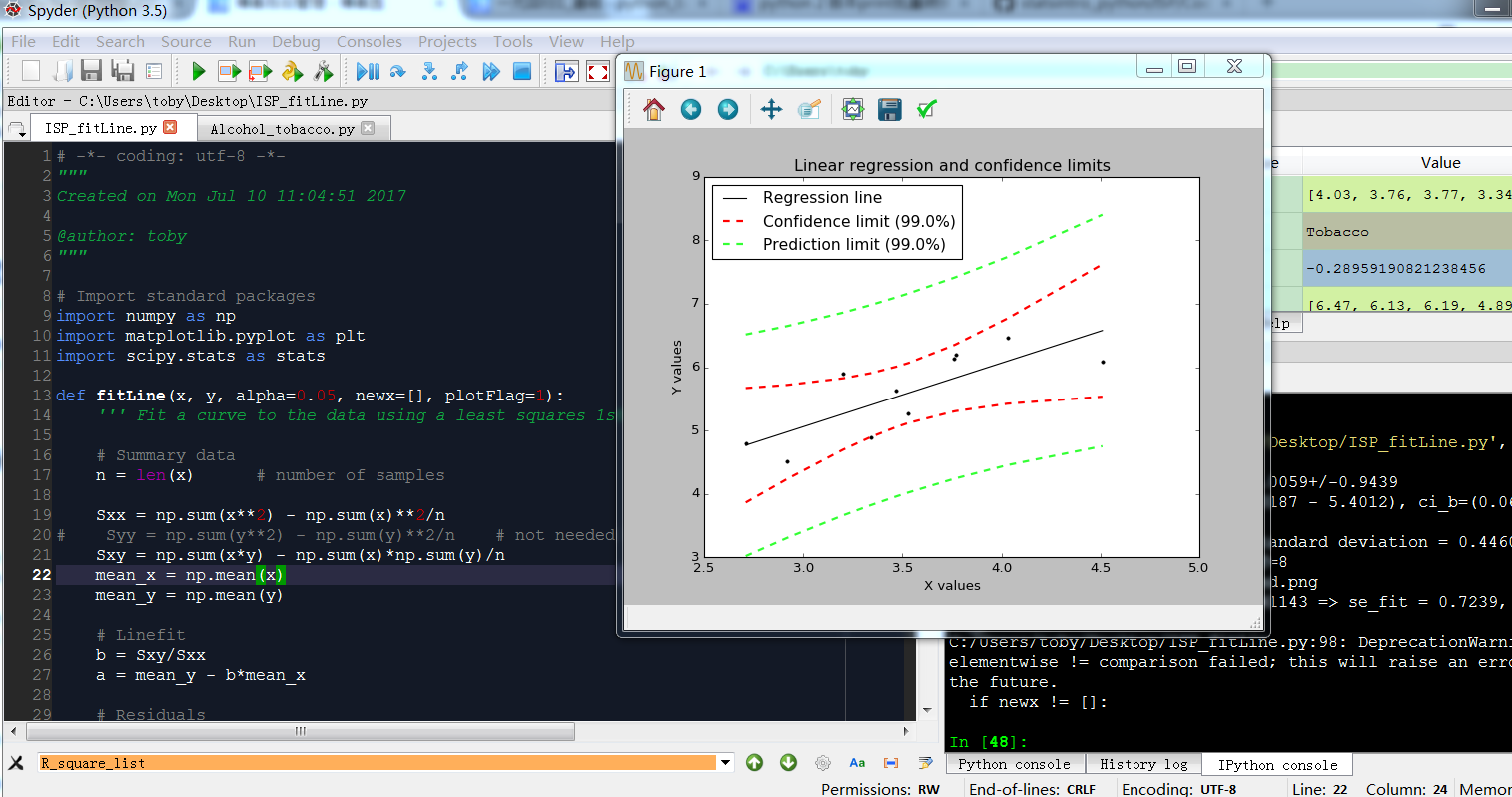
        plt.title('Linear regression and confidence limits')
        
        # configure legend
        plt.legend(loc=0)
        leg = plt.gca().get_legend()
        ltext = leg.get_texts()
        plt.setp(ltext, fontsize=14)

        # show the plot
        outFile = 'regression_wLegend.png'
        plt.savefig(outFile, dpi=200)
        print('Image saved to {0}'.format(outFile))
        plt.show()
        
    if newx != []:
        try:
            newx.size
        except AttributeError:
            newx = np.array([newx])
    
        print(('Example: x = {0}+/-{1} => se_fit = {2:5.4f}, se_predict = {3:6.5f}'
        .format(newx[0], tval*se_predict(newx[0]), se_fit(newx[0]), se_predict(newx[0]))))
        
        newy = (fit(newx), fit(newx)-se_predict(newx), fit(newx)+se_predict(newx))
        return (a,b,(ci_a, ci_b), ri, newy)
    else:
        return (a,b,(ci_a, ci_b), ri)
    

        
def Draw_confidenceInterval(x,y): 
    x=np.array(x)    
    y=np.array(y)
    goodIndex = np.invert(np.logical_or(np.isnan(x), np.isnan(y)))        
    (a,b,(ci_a, ci_b), ri,newy) = fitLine(x[goodIndex],y[goodIndex], alpha=0.01,newx=np.array([1,4.5]))   
          
y=[6.47,6.13,6.19,4.89,5.63,4.52,5.89,4.79,5.27,6.08]
x=[4.03,3.76,3.77,3.34,3.47,2.92,3.20,2.71,3.53,4.51]        

Draw_confidenceInterval(x,y)                
        

 https://study.163.com/provider/400000000398149/index.htm?share=2&shareId=400000000398149（ 欢迎关注博主主页，学习python视频资源，还有大量免费python经典文章）