zoukankan      html  css  js  c++  java
  • sklearn多分类问题

     python机器学习-乳腺癌细胞挖掘(博主亲自录制视频)

    https://study.163.com/course/introduction.htm?courseId=1005269003&utm_campaign=commission&utm_source=cp-400000000398149&utm_medium=share

    sklearnmulticlass与multilabel,one-vs-rest与one-vs-one

    针对多类问题的分类中,具体讲有两种,即multiclass classification和multilabel classification。multiclass是指分类任务中包含不止一个类别时,每条数据仅仅对应其中一个类别,不会对应多个类别。multilabel是指分类任务中不止一个分类时,每条数据可能对应不止一个类别标签,例如一条新闻,可以被划分到多个板块。

    无论是multiclass,还是multilabel,做分类时都有两种策略,一个是one-vs-​the-rest(one-vs-all),一个是one-vs-one。这个在之前的SVM介绍中(http://blog.sina.com.cn/s/blog_7103b28a0102w07f.html)也提到过。

    在one-vs-all策略中,假设有n个类别,那么就会建立n个二项分类器,每个分类器针对其中一个类别和剩余类别进行分类。进行预测时,利用这n个二项分类器进行分类,得到数据属于当前类的概率,选择其中概率最大的一个类别作为最终的预测结果。

    在one-vs-one策略中,同样假设有n个类别,则会针对两两类别建立二项分类器,得到k=n*(n-1)/2个分类器。对新数据进行分类时,依次使用这k个分类器进行分类,每次分类相当于一次投票,分类结果是哪个就相当于对哪个类投了一票。在使用全部k个分类器进行分类后,相当于进行了k次投票,选择得票最多的那个类作为最终分类结果​。

    ​在scikit-learn框架中,分别有sklearn.multiclass.OneVsRestClassifier和sklearn.multiclass.OneVsOneClassifier完成两种策略,使用过程中要指明使用的二项分类器是什么。另外在进行mutillabel分类时,训练数据的类别标签Y应该是一个矩阵,第[i,j]个元素指明了第j个类别标签是否出现在第i个样本数据中。例如,np.array([[1, 0, 0], [0, 1, 1], [0, 0, 0]]),这样的一条数据,指明针对第一条样本数据,类别标签是第0个类,第二条数据,类别标签是第1,第2个类,第三条数据,没有类别标签。有时训练数据中,类别标签Y可能不是这样的可是,而是类似[[2, 3, 4], [2], [0, 1, 3], [0, 1, 2, 3, 4], [0, 1, 2]]这样的格式,每条数据指明了每条样本数据对应的类标号。这就需要将Y转换成矩阵的形式,sklearn.preprocessing.MultiLabelBinarizer提供了这个功能。

    ​ons-vs-all的multiclass例子如下:

    ​one-vs-one的multiclass例子如下:


    https://www.cnblogs.com/taceywong/p/5932682.html


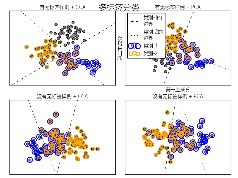
    本例模拟一个多标签文档分类问题.数据集基于下面的处理随机生成:

    • 选取标签的数目:泊松(n~Poisson,n_labels)
    • n次,选取类别C:多项式(c~Multinomial,theta)
    • 选取文档长度:泊松(k~Poisson,length)
    • k次,选取一个单词:多项式(w~Multinomial,theta_c)

    在上面的处理中,拒绝抽样用来确保n大于2,文档长度不为0.同样,我们拒绝已经被选取的类别.被同事分配给两个分类的文档会被两个圆环包围.

    通过投影到由PCA和CCA选取进行可视化的前两个主成分进行分类.接着通过元分类器使用两个线性核的SVC来为每个分类学习一个判别模型.注意,PCA用于无监督降维,CCA用于有监督.

    注:在下面的绘制中,"无标签样例"不是说我们不知道标签(就像半监督学习中的那样),而是这些样例根本没有标签~~~

    # coding:utf-8
    
    import numpy as np
    from pylab import *
    
    from sklearn.datasets import make_multilabel_classification
    from sklearn.multiclass import OneVsRestClassifier
    from sklearn.svm import SVC
    from sklearn.preprocessing import LabelBinarizer
    from sklearn.decomposition import PCA
    from sklearn.cross_decomposition import CCA
    
    
    myfont = matplotlib.font_manager.FontProperties(fname="Microsoft-Yahei-UI-Light.ttc")
    mpl.rcParams['axes.unicode_minus'] = False


    def plot_hyperplane(clf, min_x, max_x, linestyle, label):
        # 获得分割超平面
        w = clf.coef_[0]
        a = -w[0] / w[1]
        xx = np.linspace(min_x - 5, max_x + 5)  # 确保线足够长
        yy = a * xx - (clf.intercept_[0]) / w[1]
        plt.plot(xx, yy, linestyle, label=label)
    
    
    def plot_subfigure(X, Y, subplot, title, transform):
        if transform == "pca":
            X = PCA(n_components=2).fit_transform(X)
        elif transform == "cca":
            X = CCA(n_components=2).fit(X, Y).transform(X)
        else:
            raise ValueError
    
        min_x = np.min(X[:, 0])
        max_x = np.max(X[:, 0])
    
        min_y = np.min(X[:, 1])
        max_y = np.max(X[:, 1])
    
        classif = OneVsRestClassifier(SVC(kernel='linear'))
        classif.fit(X, Y)
    
        plt.subplot(2, 2, subplot)
        plt.title(title,fontproperties=myfont)
    
        zero_class = np.where(Y[:, 0])
        one_class = np.where(Y[:, 1])
        plt.scatter(X[:, 0], X[:, 1], s=40, c='gray')
        plt.scatter(X[zero_class, 0], X[zero_class, 1], s=160, edgecolors='b',
                   facecolors='none', linewidths=2, label=u'类别-1')
        plt.scatter(X[one_class, 0], X[one_class, 1], s=80, edgecolors='orange',
                   facecolors='none', linewidths=2, label=u'类别-2')
    
        plot_hyperplane(classif.estimators_[0], min_x, max_x, 'k--',
                        u'类别-1的
    边界')
        plot_hyperplane(classif.estimators_[1], min_x, max_x, 'k-.',
                        u'类别-2的
    边界')
        plt.xticks(())
        plt.yticks(())
    
        plt.xlim(min_x - .5 * max_x, max_x + .5 * max_x)
        plt.ylim(min_y - .5 * max_y, max_y + .5 * max_y)
        if subplot == 2:
            plt.xlabel(u'第一主成分',fontproperties=myfont)
            plt.ylabel(u'第二主成分',fontproperties=myfont)
            plt.legend(loc="upper left",prop=myfont)
    
    
    plt.figure(figsize=(8, 6))
    
    X, Y = make_multilabel_classification(n_classes=2, n_labels=1,
                                          allow_unlabeled=True,
                                          random_state=1)
    
    plot_subfigure(X, Y, 1, u"有无标签样例 + CCA", "cca")
    plot_subfigure(X, Y, 2, u"有无标签样例 + PCA", "pca")
    
    X, Y = make_multilabel_classification(n_classes=2, n_labels=1,
                                          allow_unlabeled=False,
                                          random_state=1)
    
    plot_subfigure(X, Y, 3, u"没有无标签样例 + CCA", "cca")
    plot_subfigure(X, Y, 4, u"没有无标签样例 + PCA", "pca")
    
    plt.subplots_adjust(.04, .02, .97, .94, .09, .2)
    plt.suptitle(u"多标签分类", size=20,fontproperties=myfont)
    plt.show()


    https://www.cnblogs.com/hapjin/p/6085278.html

    # logistics 多分类

    复制代码
    import pandas as pd
    df=pd.read_csv("logistic_data/train.tsv",header=0,delimiter='	')
    print df.count()
    print df.head()
    df.Phrase.head(10)
    df.Sentiment.describe()
    df.Sentiment.value_counts()
    df.Sentiment.value_counts()/df.Sentiment.count()
    复制代码
    复制代码
    import pandas as pd
    from sklearn.feature_extraction.text import TfidfVectorizer
    from sklearn.linear_model.logistic import LogisticRegression
    from sklearn.cross_validation import train_test_split
    from sklearn.metrics import classification_report,accuracy_score,confusion_matrix
    from sklearn.pipeline import Pipeline
    from sklearn.grid_search import GridSearchCV
    
    pipeline=Pipeline([
            ('vect',TfidfVectorizer(stop_words='english')),
            ('clf',LogisticRegression())])
    parameters={
                'vect__max_df':(0.25,0.5),
                'vect__ngram_range':((1,1),(1,2)),
                'vect__use_idf':(True,False),
                'clf__C':(0.1,1,10),
               }
    df=pd.read_csv("logistic_data/train.tsv",header=0,delimiter='	')
    X,y=df.Phrase,df.Sentiment.as_matrix()
    X_train,X_test,y_train,y_test=train_test_split(X,y,train_size=0.5)
    grid_search=GridSearchCV(pipeline,parameters,n_jobs=-1,verbose=1,scoring="accuracy")
    grid_search.fit(X_train,y_train)
    print u'最佳效果:%0.3f'%grid_search.best_score_
    print u'最优参数组合:'
    best_parameters=grid_search.best_estimator_.get_params()
    for param_name in sorted(parameters.keys()):
        print '	%s:%r'%(param_name,best_parameters[param_name])
    复制代码

    数据结果:

    Fitting 3 folds for each of 24 candidates, totalling 72 fits
    
     [Parallel(n_jobs=-1)]: Done 46 tasks | elapsed: 2.0min [Parallel(n_jobs=-1)]: Done 72 out of 72 | elapsed: 4.5min finished
     最佳效果:0.619 最优参数组合: clf__C:10 vect__max_df:0.25 vect__ngram_range:(1, 2) vect__use_idf:False

     ## 多类分类效果评估

    predictions=grid_search.predict(X_test)
    print u'准确率',accuracy_score(y_test,predictions)
    print u'混淆矩阵',confusion_matrix(y_test,predictions)
    print u'分类报告',classification_report(y_test,predictions)

    数据结果:

    准确率 0.636614122773
    混淆矩阵 [[ 1133  1712   595    67     1]
    [  919  6136  6006   553    35]
    [  213  3212 32637  3634   138]
    [   22   420  6548  8155  1274]
    [    4    45   546  2411  1614]]
    分类报告              precision    recall  f1-score   support

              0       0.49      0.32      0.39      3508
              1       0.53      0.45      0.49     13649
              2       0.70      0.82      0.76     39834
              3       0.55      0.50      0.52     16419
              4       0.53      0.35      0.42      4620

    avg / total       0.62      0.64      0.62     78030


    1.11 多分类、多标签分类

    包:sklearn.multiclass

    • OneVsRestClassifier:1-rest多分类(多标签)策略
    • OneVsOneClassifier:1-1多分类策略
    • OutputCodeClassifier:1个类用一个二进制码表示
      示例代码
    #coding=utf-8
    from sklearn import metrics
    from sklearn import cross_validation
    from sklearn.svm import SVC
    from sklearn.multiclass import OneVsRestClassifier
    from sklearn.preprocessing import MultiLabelBinarizer
    import numpy as np
    from numpy import random
    X=np.arange(15).reshape(5,3)
    y=np.arange(5)
    Y_1 = np.arange(5)
    random.shuffle(Y_1)
    Y_2 = np.arange(5)
    random.shuffle(Y_2)
    Y = np.c_[Y_1,Y_2]
    def multiclassSVM():
        X_train, X_test, y_train, y_test = cross_validation.train_test_split(X, y, test_size=0.2,random_state=0)
        model = OneVsRestClassifier(SVC())
        model.fit(X_train, y_train)
        predicted = model.predict(X_test)
        print predicted
    def multilabelSVM():
        Y_enc = MultiLabelBinarizer().fit_transform(Y)
        X_train, X_test, Y_train, Y_test = cross_validation.train_test_split(X, Y_enc, test_size=0.2, random_state=0)
        model = OneVsRestClassifier(SVC())
        model.fit(X_train, Y_train)
        predicted = model.predict(X_test)
        print predicted
    if __name__ == '__main__':
        multiclassSVM()
        # multilabelSVM()
    

    上面的代码测试了svm在OneVsRestClassifier的包装下,分别处理多分类和多标签的情况。特别注意,在多标签的情况下,输入必须是二值化的。所以需要MultiLabelBinarizer()先处理。

    2 具体模型

    2.1 朴素贝叶斯(Naive Bayes)

    包:sklearn.cross_validation

     
    朴素贝叶斯.png

    朴素贝叶斯的特点是分类速度快,分类效果不一定是最好的。

    • GasussianNB:高斯分布的朴素贝叶斯
    • MultinomialNB:多项式分布的朴素贝叶斯
    • BernoulliNB:伯努利分布的朴素贝叶斯

    所谓使用什么分布的朴素贝叶斯,就是假设P(x_i|y)是符合哪一种分布,比如可以假设其服从高斯分布,然后用最大似然法估计高斯分布的参数。

     
    高斯分布.png
     
    多项式分布.png
     
    伯努利分布.png

    3 scikit-learn扩展

    3.0 概览

    具体的扩展,通常要继承sklearn.base包下的类。

    • BaseEstimator: 估计器的基类
    • ClassifierMixin :分类器的混合类
    • ClusterMixin:聚类器的混合类
    • RegressorMixin :回归器的混合类
    • TransformerMixin :转换器的混合类

    关于什么是Mixin(混合类),具体可以看这个知乎链接。简单地理解,就是带有实现方法的接口,可以将其看做是组合模式的一种实现。举个例子,比如说常用的TfidfTransformer,继承了BaseEstimator, TransformerMixin,因此它的基本功能就是单一职责的估计器和转换器的组合。

    3.1 创建自己的转换器

    在特征抽取的时候,经常会发现自己的一些数据预处理的方法,sklearn里可能没有实现,但若直接在数据上改,又容易将代码弄得混乱,难以重现实验。这个时候最好自己创建一个转换器,在后面将这个转换器放到pipeline里,统一管理。
    例如《Python数据挖掘入门与实战》书中的例子,我们想接收一个numpy数组,根据其均值将其离散化,任何高于均值的特征值替换为1,小于或等于均值的替换为0。
    代码实现:

    from sklearn.base import TransformerMixin
    from sklearn.utils import as_float_array
    
    class MeanDiscrete(TransformerMixin):
      
      #计算出数据集的均值,用内部变量保存该值。  
      def fit(self, X, y=None):
            X = as_float_array(X)
            self.mean = np.mean(X, axis=0)
            #返回self,确保在转换器中能够进行链式调用(例如调用transformer.fit(X).transform(X))
            return self
    
        def transform(self, X):
            X = as_float_array(X)
            assert X.shape[1] == self.mean.shape[0]
            return X > self.mean


    作者:Cer_ml
    链接:https://www.jianshu.com/p/516f009c0875
    來源:简书
    著作权归作者所有。商业转载请联系作者获得授权,非商业转载请注明出处。


    sklearn学习笔记(3)svm多分类

    http://blog.csdn.net/babybirdtofly/article/details/72886879

    SVC、NuSVC、LinearSVC都可以在一个数据集上实现多分类。 
    SVC和NuSVC方法类似,但是有不同的输入参数集和不同的数学表述。另一方面,linearSVC是SVC的在线性核的基础上的另一种实现,所以LinearSVC不能不能接受关键字“kernel”,只能是线性。 
    二分类 
    和别的分类器一样,三种分类器需要输入两个数组:X[n样本][n维特征](训练数据集)Y[n个标签](类标签)

    from sklearn import svm
    X = [[0,0], [1,1]]
    Y = [0, 1]
    • 1
    • 2
    • 3

    模型学习之后可以进行预测:

    clf = svm.SVC()
    clf.fit(X,y)
    clf.predict([[2.,2.]])
    • 1
    • 2
    • 3

    SVM的决策函数依赖于训练数据集的支持向量子集。这些属性可以通过下面函数进行查看

    #get support vector
    clf.support_vectors_
    #get indices of support vectors
    clf.support_
    #get number of support vectors for each class
    clf.n_support_
    • 1
    • 2
    • 3
    • 4
    • 5
    • 6

    多分类 
    SVC和NuSVC实现“1v1“的方法进行多分类(Knerr et al,1990)。如果n_class是类别的数量,那么需要建立n*n/2个分类器,desision_function_shape选项允许集成“1v1”分类器来刻画(n_samples,n_features

    clf = svm.SVC(decision_function_shape='ovo')
    clf.fit(X, Y)
    dec = clf.decision_function([[1]])
    print dec.shape[1] # 4 classes: 4*3/2 = 6
    print clf.predict([[1]])
    
    clf.decision_function_shape = "ovr"
    dec = clf.decision_function([[1]])
    print dec.shape[1]
    print clf.predict([[2.4]])
    • 1
    • 2
    • 3
    • 4
    • 5
    • 6
    • 7
    • 8
    • 9
    • 10

    同时,LinearSVC也实现了“one vs the rest”多分类策略。

    lin_clf = svm.LinearSVC()
    lin_clf.fit(X,Y)
    dec = lin_clf.decision_function([[3]])
    print dec.shape[1]
    print lin_clf.predict(2.4)
    • 1
    • 2
    • 3
    • 4
    • 5

    评分和概率 
    SVC方法decision_function给每个样本中的每个类一个评分,当我们将probability设置为True之后,我们可以通过predict_probapredict_log_proba可以对类别概率进行评估。 
    Wu, Lin and Weng, “Probability estimates for multi-class classification by pairwise coupling”, JMLR 5:975-1005, 2004. 
    不均衡问题 
    我们可以通过class_weightsample_weight两个关键字实现对特定类别或者特定样本的权重调整。


    本作业使用逻辑回归(logistic regression)和神经网络(neural networks)识别手写的阿拉伯数字(0-9)

    关于逻辑回归的一个编程练习,可参考:Stanford coursera Andrew Ng 机器学习课程编程作业(Exercise 2)及总结

    下面使用逻辑回归实现多分类问题:识别手写的阿拉伯数字(0-9),使用神经网络实现:识别手写的阿拉伯数字(0-9),请参考:神经网络实现


    数据加载到Matlab中的格式如下:


    一共有5000个训练样本,每个训练样本是400维的列向量(20X20像素的 grayscale image),用矩阵 X 保存。样本的结果(label of training set)保存在向量 y 中,y 是一个5000行1列的列向量。

    比如 y = (1,2,3,4,5,6,7,8,9,10......)T,注意,由于Matlab下标是从1开始的,故用 10 表示数字 0


    ①样本数据的可视化

    随机选择100个样本数据,使用Matlab可视化的结果如下:

     
    ②使用逻辑回归来实现多分类问题(one-vs-all)

    所谓多分类问题,是指分类的结果为三类以上。比如,预测明天的天气结果为三类:晴(用y==1表示)、阴(用y==2表示)、雨(用y==3表示)

    分类的思想,其实与逻辑回归分类(默认是指二分类,binary classification)很相似,对“晴天”进行分类时,将另外两类(阴天和下雨)视为一类:(非晴天),这样,就把一个多分类问题转化成了二分类问题。示意图如下:(图中的圆圈 表示:不属于某一类的 所有其他类)


    对于N分类问题(N>=3),就需要N个假设函数(预测模型),也即需要N组模型参数θ(θ一般是一个向量)

    然后,对于每个样本实例,依次使用每个模型预测输出,选取输出值最大的那组模型所对应的预测结果作为最终结果。

    因为模型的输出值,在sigmoid函数作用下,其实是一个概率值。,注意:hθ(1)(x),hθ(2)(x),hθ(3)(x)三组 模型参数θ 一般是不同的。比如:

    hθ(1)(x),输出 预测为晴天(y==1)的概率

    hθ(2)(x),输出 预测为阴天(y==2)的概率

    hθ(3)(x),输出 预测为雨天(y==3)的概率


    ③Matlab代码实现

    对于上面的识别阿拉伯数字的问题,一共需要训练出10个逻辑回归模型,每个逻辑回归模型对应着识别其中一个数字。

    我们一共有5000个样本,样本的预测结果值就是:y=(1,2,3,4,5,6,7,8,9,10),其中 10 代表 数字0

    我们使用Matlab fmincg库函数 来求解使得代价函数取最小值的 模型参数θ

    复制代码
    function [all_theta] = oneVsAll(X, y, num_labels, lambda)
    %ONEVSALL trains multiple logistic regression classifiers and returns all
    %the classifiers in a matrix all_theta, where the i-th row of all_theta 
    %corresponds to the classifier for label i
    %   [all_theta] = ONEVSALL(X, y, num_labels, lambda) trains num_labels
    %   logisitc regression classifiers and returns each of these classifiers
    %   in a matrix all_theta, where the i-th row of all_theta corresponds 
    %   to the classifier for label i
    
    % Some useful variables
    m = size(X, 1);% num of samples
    n = size(X, 2);% num of features
    
    % You need to return the following variables correctly 
    all_theta = zeros(num_labels, n + 1);
    
    % Add ones to the X data matrix
    X = [ones(m, 1) X];
    
    % ====================== YOUR CODE HERE ======================
    % Instructions: You should complete the following code to train num_labels
    %               logistic regression classifiers with regularization
    %               parameter lambda. 
    %
    % Hint: theta(:) will return a column vector.
    %
    % Hint: You can use y == c to obtain a vector of 1's and 0's that tell use 
    %       whether the ground truth is true/false for this class.
    %
    % Note: For this assignment, we recommend using fmincg to optimize the cost
    %       function. It is okay to use a for-loop (for c = 1:num_labels) to
    %       loop over the different classes.
    %
    %       fmincg works similarly to fminunc, but is more efficient when we
    %       are dealing with large number of parameters.
    %
    % Example Code for fmincg:
    %
    %     % Set Initial theta
    %     initial_theta = zeros(n + 1, 1);
    %     
    %     % Set options for fminunc
    %     options = optimset('GradObj', 'on', 'MaxIter', 50);
    % 
    %     % Run fmincg to obtain the optimal theta
    %     % This function will return theta and the cost 
    %     [theta] = ...
    %         fmincg (@(t)(lrCostFunction(t, X, (y == c), lambda)), ...
    %                 initial_theta, options);
    %
    initial_theta = zeros(n + 1, 1);
    
    options = optimset('GradObj','on','MaxIter',50);
    
    for c = 1:num_labels %num_labels 为逻辑回归训练器的个数,num of logistic regression classifiers
    all_theta(c, :) = fmincg(@(t)(lrCostFunction(t, X, (y == c),lambda)), initial_theta,options );
    end
    % =========================================================================
    end
    复制代码

    lrCostFunction,完全可参考:http://www.cnblogs.com/hapjin/p/6078530.html 里面的 正则化的逻辑回归模型实现costFunctionReg.m文件


    下面来解释一下 for循环:

    num_labels 为分类器个数,共10个,每个分类器(模型)用来识别10个数字中的某一个。

    我们一共有5000个样本,每个样本有400中特征变量,因此:模型参数θ 向量有401个元素。

    initial_theta = zeros(n + 1, 1); % 模型参数θ的初始值(n == 400)

    all_theta是一个10*401的矩阵,每一行存储着一个分类器(模型)的模型参数θ 向量,执行上面for循环,就调用fmincg库函数 求出了 所有模型的参数θ 向量了。


    求出了每个模型的参数向量θ,就可以用 训练好的模型来识别数字了。对于一个给定的数字输入(400个 feature variables) input instance,每个模型的假设函数hθ(i)(x) 输出一个值(i = 1,2,...10)。取这10个值中最大值那个值,作为最终的识别结果。比如g(hθ(8)(x))==0.96 比其它所有的 g(hθ(i)(x)) (i = 1,2,...10,但 i 不等于8) 都大,则识别的结果为 数字 8


    复制代码
    function p = predictOneVsAll(all_theta, X)
    %PREDICT Predict the label for a trained one-vs-all classifier. The labels 
    %are in the range 1..K, where K = size(all_theta, 1). 
    %  p = PREDICTONEVSALL(all_theta, X) will return a vector of predictions
    %  for each example in the matrix X. Note that X contains the examples in
    %  rows. all_theta is a matrix where the i-th row is a trained logistic
    %  regression theta vector for the i-th class. You should set p to a vector
    %  of values from 1..K (e.g., p = [1; 3; 1; 2] predicts classes 1, 3, 1, 2
    %  for 4 examples) 
    
    m = size(X, 1);
    num_labels = size(all_theta, 1);
    
    % You need to return the following variables correctly 
    p = zeros(size(X, 1), 1);
    
    % Add ones to the X data matrix
    X = [ones(m, 1) X];
    
    % ====================== YOUR CODE HERE ======================
    % Instructions: Complete the following code to make predictions using
    %               your learned logistic regression parameters (one-vs-all).
    %               You should set p to a vector of   (from 1 to
    %               num_labels).
    %
    % Hint: This code can be done all vectorized using the max function.
    %       In particular, the max function can also return the index of the 
    %       max element, for more information see 'help max'. If your examples 
    %       are in rows, then, you can use max(A, [], 2) to obtain the max 
    %       for each row.
    %       
    
    [~,p] = max( X * all_theta',[],2); % 求矩阵(X*all_theta')每行的最大值,p 记录矩阵每行的最大值的索引
    % =========================================================================
    end


     https://study.163.com/provider/400000000398149/index.htm?share=2&shareId=400000000398149( 欢迎关注博主主页,学习python视频资源,还有大量免费python经典文章)


  • 相关阅读:
    jquery animate()方法 语法
    jquery unload方法 语法
    jquery undelegate()方法 语法
    jquery unbind()方法 语法
    jquery trigger() 方法 语法
    jquery toggle()方法 语法
    jquery change() 函数 语法
    jquery blur()函数 语法
    jquery bind()方法 语法
    jquery checked选择器 语法
  • 原文地址:https://www.cnblogs.com/webRobot/p/8417364.html
Copyright © 2011-2022 走看看