zoukankan html css js c++ java

sklearn—特征工程

sklearn实战-乳腺癌细胞数据挖掘（博主亲自录制视频）

https://study.163.com/course/introduction.htm?courseId=1005269003&utm_campaign=commission&utm_source=cp-400000000398149&utm_medium=share

项目合作QQ：231469242

变量筛选：（逻辑回归）

好处：

变量少，模型运行速度快，更容易解读和理解

坏处：

会牺牲掉少量精确性

变量不筛选：（random forest）

好处：

提高准确性

坏处：

变量多，运行速度慢

logistic模型为什么要考虑共线性问题？
共线性问题会导致估计结果不准确，系数方向都可能发生改变。不管是logistic回归模型，还是ols都要考虑。

官网

http://scikit-learn.org/stable/modules/feature_selection.html

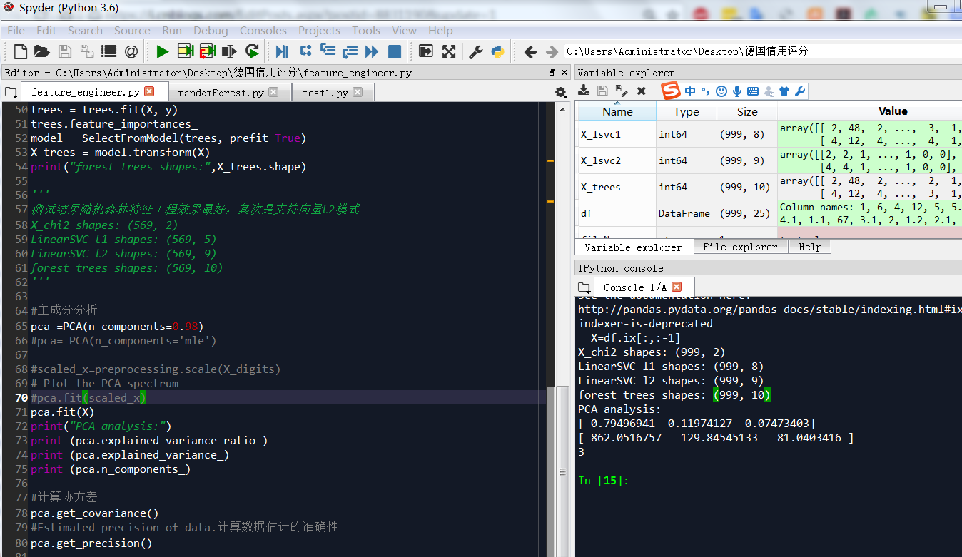
测试结果随机森林特征工程效果最好，其次是支持向量l2模式

主成分一个就可以解释98%以上方差，和spss结果差距大，需要核实

# -*- coding: utf-8 -*-
"""
Created on Sat Apr 14 19:36:29 2018

@author: Administrator
#乳腺癌数据测试中，卡方检验效果不如随机森林,卡方筛选的2个最好因子在随机森林中权重不是最大

"""
from sklearn.decomposition import PCA
from sklearn.ensemble import ExtraTreesClassifier
from sklearn.feature_selection import SelectFromModel
from sklearn.datasets import load_breast_cancer
from sklearn.feature_selection import SelectKBest
from sklearn.feature_selection import chi2
from sklearn.svm import LinearSVC
cancer = load_breast_cancer()
X= cancer.data
y= cancer.target

#特征工程-卡方筛选K个最佳特征
#乳腺癌数据测试中，卡方检验效果不如随机森林,卡方筛选的2个最好因子在随机森林中权重不是最大
#we can perform a chi^2 test to the samples to retrieve only the two best features as follows:
X_chi2 = SelectKBest(chi2, k=2).fit_transform(X, y)
print("X_chi2 shapes:",X_chi2.shape) 

##特征工程-支持向量l1
#根据模型选择最佳特征，线性svc选出5个最佳特征
lsvc = LinearSVC(C=0.01, penalty="l1", dual=False).fit(X, y)
model = SelectFromModel(lsvc, prefit=True)
X_lsvc1 = model.transform(X)
print("LinearSVC l1 shapes:",X_lsvc1.shape) 

#特征工程-支持向量l2
lsvc = LinearSVC(C=0.01, penalty="l2", dual=False).fit(X, y)
model = SelectFromModel(lsvc, prefit=True)
X_lsvc2 = model.transform(X)
print("LinearSVC l2 shapes:",X_lsvc2.shape) 

#特征工程-forest of trees 随机森林
trees = ExtraTreesClassifier(n_estimators=10000)
trees = trees.fit(X, y)
trees.feature_importances_  
model = SelectFromModel(trees, prefit=True)
X_trees = model.transform(X)
print("forest trees shapes:",X_trees.shape) 

'''
测试结果随机森林特征工程效果最好，其次是支持向量l2模式
X_chi2 shapes: (569, 2)
LinearSVC l1 shapes: (569, 5)
LinearSVC l2 shapes: (569, 9)
forest trees shapes: (569, 10)
'''

#主成分分析
pca =PCA(n_components=0.98)
#pca= PCA(n_components='mle')

digits = load_breast_cancer()
X_digits = cancer.data
y_digits = digits.target

#scaled_x=preprocessing.scale(X_digits)
# Plot the PCA spectrum
#pca.fit(scaled_x)
pca.fit(X_digits)
print("PCA analysis:")
print (pca.explained_variance_ratio_)
print (pca.explained_variance_)
print (pca.n_components_)

#计算协方差
pca.get_covariance()
#Estimated precision of data.计算数据估计的准确性
pca.get_precision()

德国信用评分卡测试

数据必须整理为数字型，不接受分类变量

# -*- coding: utf-8 -*-
"""
Created on Sat Apr 14 19:36:29 2018

@author: Administrator
#乳腺癌数据测试中，卡方检验效果不如随机森林,卡方筛选的2个最好因子在随机森林中权重不是最大

"""
import pandas as pd
import numpy as np
from sklearn.decomposition import PCA
from sklearn.ensemble import ExtraTreesClassifier
from sklearn.feature_selection import SelectFromModel
from sklearn.feature_selection import SelectKBest
from sklearn.feature_selection import chi2
from sklearn.svm import LinearSVC
from sklearn.ensemble import RandomForestClassifier

trees=100
#读取文件
readFileName="GermanData_total.xlsx"
#读取excel
df=pd.read_excel(readFileName)
list_columns=list(df.columns[:-1])
X=df.ix[:,:-1]
y=df.ix[:,-1]
#X_dummy=pd.get_dummies(X)

#特征工程-卡方筛选K个最佳特征
#乳腺癌数据测试中，卡方检验效果不如随机森林,卡方筛选的2个最好因子在随机森林中权重不是最大
#we can perform a chi^2 test to the samples to retrieve only the two best features as follows:
X_chi2 = SelectKBest(chi2, k=2).fit_transform(X, y)
print("X_chi2 shapes:",X_chi2.shape) 

##特征工程-支持向量l1
#根据模型选择最佳特征，线性svc选出5个最佳特征
lsvc = LinearSVC(C=0.01, penalty="l1", dual=False).fit(X, y)
model = SelectFromModel(lsvc, prefit=True)
X_lsvc1 = model.transform(X)
print("LinearSVC l1 shapes:",X_lsvc1.shape) 

#特征工程-支持向量l2
lsvc = LinearSVC(C=0.01, penalty="l2", dual=False).fit(X, y)
model = SelectFromModel(lsvc, prefit=True)
X_lsvc2 = model.transform(X)
print("LinearSVC l2 shapes:",X_lsvc2.shape) 

#特征工程-forest of trees 随机森林
trees = ExtraTreesClassifier(n_estimators=10000)
trees = trees.fit(X, y)
trees.feature_importances_  
model = SelectFromModel(trees, prefit=True)
X_trees = model.transform(X)
print("forest trees shapes:",X_trees.shape) 

'''
测试结果随机森林特征工程效果最好，其次是支持向量l2模式
X_chi2 shapes: (569, 2)
LinearSVC l1 shapes: (569, 5)
LinearSVC l2 shapes: (569, 9)
forest trees shapes: (569, 10)
'''

#主成分分析
pca =PCA(n_components=0.98)
#pca= PCA(n_components='mle')

#scaled_x=preprocessing.scale(X_digits)
# Plot the PCA spectrum
#pca.fit(scaled_x)
pca.fit(X)
print("PCA analysis:")
print (pca.explained_variance_ratio_)
print (pca.explained_variance_)
print (pca.n_components_)

#计算协方差
pca.get_covariance()
#Estimated precision of data.计算数据估计的准确性
pca.get_precision()

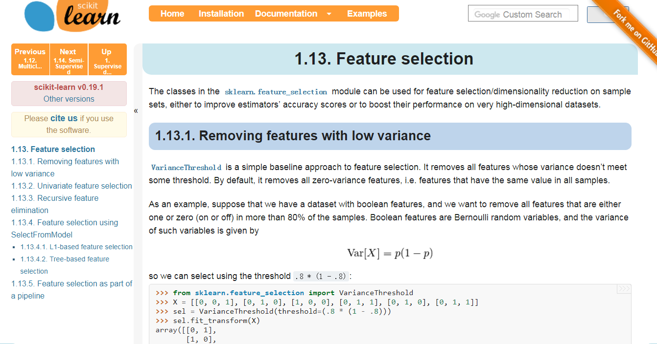
The classes in the sklearn.feature_selection module can be used for feature selection/dimensionality reduction on sample sets, either to improve estimators’ accuracy scores or to boost their performance on very high-dimensional datasets.

1.13.1. Removing features with low variance

VarianceThreshold is a simple baseline approach to feature selection. It removes all features whose variance doesn’t meet some threshold. By default, it removes all zero-variance features, i.e. features that have the same value in all samples.

As an example, suppose that we have a dataset with boolean features, and we want to remove all features that are either one or zero (on or off) in more than 80% of the samples. Boolean features are Bernoulli random variables, and the variance of such variables is given by

$mathrm{Var}[X] = p(1 - p)$

so we can select using the threshold .8 * (1 - .8):

>>>
>>> from sklearn.feature_selection import VarianceThreshold
>>> X = [[0, 0, 1], [0, 1, 0], [1, 0, 0], [0, 1, 1], [0, 1, 0], [0, 1, 1]]
>>> sel = VarianceThreshold(threshold=(.8 * (1 - .8)))
>>> sel.fit_transform(X)
array([[0, 1],
       [1, 0],
       [0, 0],
       [1, 1],
       [1, 0],
       [1, 1]])

As expected, VarianceThreshold has removed the first column, which has a probability $p = 5/6 > .8$ of containing a zero.

1.13.2. Univariate feature selection

Univariate feature selection works by selecting the best features based on univariate statistical tests. It can be seen as a preprocessing step to an estimator. Scikit-learn exposes feature selection routines as objects that implement the transformmethod:

SelectKBest removes all but the $k$ highest scoring features

SelectPercentile removes all but a user-specified highest scoring percentage of features

using common univariate statistical tests for each feature: false positive rate SelectFpr, false discovery rate SelectFdr, or family wise error SelectFwe.

GenericUnivariateSelect allows to perform univariate feature selection with a configurable strategy. This allows to select the best univariate selection strategy with hyper-parameter search estimator.

For instance, we can perform a $chi^2$ test to the samples to retrieve only the two best features as follows:

>>>
>>> from sklearn.datasets import load_iris
>>> from sklearn.feature_selection import SelectKBest
>>> from sklearn.feature_selection import chi2
>>> iris = load_iris()
>>> X, y = iris.data, iris.target
>>> X.shape
(150, 4)
>>> X_new = SelectKBest(chi2, k=2).fit_transform(X, y)
>>> X_new.shape
(150, 2)

These objects take as input a scoring function that returns univariate scores and p-values (or only scores for SelectKBestand SelectPercentile):

For regression: f_regression, mutual_info_regression

For classification: chi2, f_classif, mutual_info_classif

The methods based on F-test estimate the degree of linear dependency between two random variables. On the other hand, mutual information methods can capture any kind of statistical dependency, but being nonparametric, they require more samples for accurate estimation.

Feature selection with sparse data

If you use sparse data (i.e. data represented as sparse matrices), chi2, mutual_info_regression, mutual_info_classifwill deal with the data without making it dense.

Warning

Beware not to use a regression scoring function with a classification problem, you will get useless results.

Examples:

1.13.3. Recursive feature elimination

Given an external estimator that assigns weights to features (e.g., the coefficients of a linear model), recursive feature elimination (RFE) is to select features by recursively considering smaller and smaller sets of features. First, the estimator is trained on the initial set of features and the importance of each feature is obtained either through a coef_ attribute or through a feature_importances_ attribute. Then, the least important features are pruned from current set of features.That procedure is recursively repeated on the pruned set until the desired number of features to select is eventually reached.

RFECV performs RFE in a cross-validation loop to find the optimal number of features.

Examples:

Recursive feature elimination: A recursive feature elimination example showing the relevance of pixels in a digit classification task.
Recursive feature elimination with cross-validation: A recursive feature elimination example with automatic tuning of the number of features selected with cross-validation.

1.13.4. Feature selection using SelectFromModel

SelectFromModel is a meta-transformer that can be used along with any estimator that has a coef_ or feature_importances_attribute after fitting. The features are considered unimportant and removed, if the corresponding coef_ or feature_importances_ values are below the provided threshold parameter. Apart from specifying the threshold numerically, there are built-in heuristics for finding a threshold using a string argument. Available heuristics are “mean”, “median” and float multiples of these like “0.1*mean”.

For examples on how it is to be used refer to the sections below.

Examples

Feature selection using SelectFromModel and LassoCV: Selecting the two most important features from the Boston dataset without knowing the threshold beforehand.

1.13.4.1. L1-based feature selection

Linear models penalized with the L1 norm have sparse solutions: many of their estimated coefficients are zero. When the goal is to reduce the dimensionality of the data to use with another classifier, they can be used along with feature_selection.SelectFromModel to select the non-zero coefficients. In particular, sparse estimators useful for this purpose are the linear_model.Lasso for regression, and of linear_model.LogisticRegression and svm.LinearSVC for classification:

>>>
>>> from sklearn.svm import LinearSVC
>>> from sklearn.datasets import load_iris
>>> from sklearn.feature_selection import SelectFromModel
>>> iris = load_iris()
>>> X, y = iris.data, iris.target
>>> X.shape
(150, 4)
>>> lsvc = LinearSVC(C=0.01, penalty="l1", dual=False).fit(X, y)
>>> model = SelectFromModel(lsvc, prefit=True)
>>> X_new = model.transform(X)
>>> X_new.shape
(150, 3)

With SVMs and logistic-regression, the parameter C controls the sparsity: the smaller C the fewer features selected. With Lasso, the higher the alpha parameter, the fewer features selected.

Examples:

Classification of text documents using sparse features: Comparison of different algorithms for document classification including L1-based feature selection.

L1-recovery and compressive sensing

For a good choice of alpha, the Lasso can fully recover the exact set of non-zero variables using only few observations, provided certain specific conditions are met. In particular, the number of samples should be “sufficiently large”, or L1 models will perform at random, where “sufficiently large” depends on the number of non-zero coefficients, the logarithm of the number of features, the amount of noise, the smallest absolute value of non-zero coefficients, and the structure of the design matrix X. In addition, the design matrix must display certain specific properties, such as not being too correlated.

There is no general rule to select an alpha parameter for recovery of non-zero coefficients. It can by set by cross-validation (LassoCV or LassoLarsCV), though this may lead to under-penalized models: including a small number of non-relevant variables is not detrimental to prediction score. BIC (LassoLarsIC) tends, on the opposite, to set high values of alpha.

Reference Richard G. Baraniuk “Compressive Sensing”, IEEE Signal Processing Magazine [120] July 2007http://dsp.rice.edu/sites/dsp.rice.edu/files/cs/baraniukCSlecture07.pdf

1.13.4.2. Tree-based feature selection

Tree-based estimators (see the sklearn.tree module and forest of trees in the sklearn.ensemble module) can be used to compute feature importances, which in turn can be used to discard irrelevant features (when coupled with the sklearn.feature_selection.SelectFromModel meta-transformer):

>>>
>>> from sklearn.ensemble import ExtraTreesClassifier
>>> from sklearn.datasets import load_iris
>>> from sklearn.feature_selection import SelectFromModel
>>> iris = load_iris()
>>> X, y = iris.data, iris.target
>>> X.shape
(150, 4)
>>> clf = ExtraTreesClassifier()
>>> clf = clf.fit(X, y)
>>> clf.feature_importances_  
array([ 0.04...,  0.05...,  0.4...,  0.4...])
>>> model = SelectFromModel(clf, prefit=True)
>>> X_new = model.transform(X)
>>> X_new.shape               
(150, 2)

Examples:

Feature importances with forests of trees: example on synthetic data showing the recovery of the actually meaningful features.
Pixel importances with a parallel forest of trees: example on face recognition data.

1.13.5. Feature selection as part of a pipeline

Feature selection is usually used as a pre-processing step before doing the actual learning. The recommended way to do this in scikit-learn is to use a sklearn.pipeline.Pipeline:

clf = Pipeline([
  ('feature_selection', SelectFromModel(LinearSVC(penalty="l1"))),
  ('classification', RandomForestClassifier())
])
clf.fit(X, y)

In this snippet we make use of a sklearn.svm.LinearSVC coupled with sklearn.feature_selection.SelectFromModel to evaluate feature importances and select the most relevant features. Then, a sklearn.ensemble.RandomForestClassifier is trained on the transformed output, i.e. using only relevant features. You can perform similar operations with the other feature selection methods and also classifiers that provide a way to evaluate feature importances of course. See the sklearn.pipeline.Pipeline examples for more details.

https://www.cnblogs.com/jasonfreak/p/5448385.html

一个懒惰的人，总是想设计更智能的程序来避免做重复性工作

1 特征工程是什么？
2 数据预处理
　　2.1 无量纲化
　　　　2.1.1 标准化
　　　　2.1.2 区间缩放法
　　　　2.1.3 标准化与归一化的区别
　　2.2 对定量特征二值化
　　2.3 对定性特征哑编码
　　2.4 缺失值计算
　　2.5 数据变换
　　2.6 回顾
3 特征选择
　　3.1 Filter
　　　　3.1.1 方差选择法
　　　　3.1.2 相关系数法
　　　　3.1.3 卡方检验
　　　　3.1.4 互信息法
　　3.2 Wrapper
　　　　3.2.1 递归特征消除法
　　3.3 Embedded
　　　　3.3.1 基于惩罚项的特征选择法
　　　　3.3.2 基于树模型的特征选择法
　　3.4 回顾
4 降维
　　4.1 主成分分析法（PCA）
　　4.2 线性判别分析法（LDA）
　　4.3 回顾
5 总结
6 参考资料

1 特征工程是什么？

　　有这么一句话在业界广泛流传：数据和特征决定了机器学习的上限，而模型和算法只是逼近这个上限而已。那特征工程到底是什么呢？顾名思义，其本质是一项工程活动，目的是最大限度地从原始数据中提取特征以供算法和模型使用。通过总结和归纳，人们认为特征工程包括以下方面：

　　特征处理是特征工程的核心部分，sklearn提供了较为完整的特征处理方法，包括数据预处理，特征选择，降维等。首次接触到sklearn，通常会被其丰富且方便的算法模型库吸引，但是这里介绍的特征处理库也十分强大！

　　本文中使用sklearn中的IRIS（鸢尾花）数据集来对特征处理功能进行说明。IRIS数据集由Fisher在1936年整理，包含4个特征（Sepal.Length（花萼长度）、Sepal.Width（花萼宽度）、Petal.Length（花瓣长度）、Petal.Width（花瓣宽度）），特征值都为正浮点数，单位为厘米。目标值为鸢尾花的分类（Iris Setosa（山鸢尾）、Iris Versicolour（杂色鸢尾），Iris Virginica（维吉尼亚鸢尾））。导入IRIS数据集的代码如下：

 1 from sklearn.datasets import load_iris
 2 
 3 #导入IRIS数据集
 4 iris = load_iris()
 5 
 6 #特征矩阵
 7 iris.data
 8 
 9 #目标向量
10 iris.target

2 数据预处理

　　通过特征提取，我们能得到未经处理的特征，这时的特征可能有以下问题：

不属于同一量纲：即特征的规格不一样，不能够放在一起比较。无量纲化可以解决这一问题。
信息冗余：对于某些定量特征，其包含的有效信息为区间划分，例如学习成绩，假若只关心“及格”或不“及格”，那么需要将定量的考分，转换成“1”和“0”表示及格和未及格。二值化可以解决这一问题。
定性特征不能直接使用：某些机器学习算法和模型只能接受定量特征的输入，那么需要将定性特征转换为定量特征。最简单的方式是为每一种定性值指定一个定量值，但是这种方式过于灵活，增加了调参的工作。通常使用哑编码的方式将定性特征转换为定量特征：假设有N种定性值，则将这一个特征扩展为N种特征，当原始特征值为第i种定性值时，第i个扩展特征赋值为1，其他扩展特征赋值为0。哑编码的方式相比直接指定的方式，不用增加调参的工作，对于线性模型来说，使用哑编码后的特征可达到非线性的效果。
存在缺失值：缺失值需要补充。
信息利用率低：不同的机器学习算法和模型对数据中信息的利用是不同的，之前提到在线性模型中，使用对定性特征哑编码可以达到非线性的效果。类似地，对定量变量多项式化，或者进行其他的转换，都能达到非线性的效果。

　　我们使用sklearn中的preproccessing库来进行数据预处理，可以覆盖以上问题的解决方案。

2.1 无量纲化

　　无量纲化使不同规格的数据转换到同一规格。常见的无量纲化方法有标准化和区间缩放法。标准化的前提是特征值服从正态分布，标准化后，其转换成标准正态分布。区间缩放法利用了边界值信息，将特征的取值区间缩放到某个特点的范围，例如[0, 1]等。

2.1.1 标准化

　　标准化需要计算特征的均值和标准差，公式表达为：

　　使用preproccessing库的StandardScaler类对数据进行标准化的代码如下：

1 from sklearn.preprocessing import StandardScaler
2 
3 #标准化，返回值为标准化后的数据
4 StandardScaler().fit_transform(iris.data)

2.1.2 区间缩放法

　　区间缩放法的思路有多种，常见的一种为利用两个最值进行缩放，公式表达为：

　　使用preproccessing库的MinMaxScaler类对数据进行区间缩放的代码如下：

1 from sklearn.preprocessing import MinMaxScaler
2 
3 #区间缩放，返回值为缩放到[0, 1]区间的数据
4 MinMaxScaler().fit_transform(iris.data)

2.1.3 标准化与归一化的区别

　　简单来说，标准化是依照特征矩阵的列处理数据，其通过求z-score的方法，将样本的特征值转换到同一量纲下。归一化是依照特征矩阵的行处理数据，其目的在于样本向量在点乘运算或其他核函数计算相似性时，拥有统一的标准，也就是说都转化为“单位向量”。规则为l2的归一化公式如下：

　　使用preproccessing库的Normalizer类对数据进行归一化的代码如下：

1 from sklearn.preprocessing import Normalizer
2 
3 #归一化，返回值为归一化后的数据
4 Normalizer().fit_transform(iris.data)

2.2 对定量特征二值化

　　定量特征二值化的核心在于设定一个阈值，大于阈值的赋值为1，小于等于阈值的赋值为0，公式表达如下：

　　使用preproccessing库的Binarizer类对数据进行二值化的代码如下：

1 from sklearn.preprocessing import Binarizer
2 
3 #二值化，阈值设置为3，返回值为二值化后的数据
4 Binarizer(threshold=3).fit_transform(iris.data)

2.3 对定性特征哑编码

　　由于IRIS数据集的特征皆为定量特征，故使用其目标值进行哑编码（实际上是不需要的）。使用preproccessing库的OneHotEncoder类对数据进行哑编码的代码如下：

1 from sklearn.preprocessing import OneHotEncoder
2 
3 #哑编码，对IRIS数据集的目标值，返回值为哑编码后的数据
4 OneHotEncoder().fit_transform(iris.target.reshape((-1,1)))

2.4 缺失值计算

　　由于IRIS数据集没有缺失值，故对数据集新增一个样本，4个特征均赋值为NaN，表示数据缺失。使用preproccessing库的Imputer类对数据进行缺失值计算的代码如下：

1 from numpy import vstack, array, nan
2 from sklearn.preprocessing import Imputer
3 
4 #缺失值计算，返回值为计算缺失值后的数据
5 #参数missing_value为缺失值的表示形式，默认为NaN
6 #参数strategy为缺失值填充方式，默认为mean（均值）
7 Imputer().fit_transform(vstack((array([nan, nan, nan, nan]), iris.data)))

2.5 数据变换

　　常见的数据变换有基于多项式的、基于指数函数的、基于对数函数的。4个特征，度为2的多项式转换公式如下：

　　使用preproccessing库的PolynomialFeatures类对数据进行多项式转换的代码如下：

1 from sklearn.preprocessing import PolynomialFeatures
2 
3 #多项式转换
4 #参数degree为度，默认值为2
5 PolynomialFeatures().fit_transform(iris.data)

　　基于单变元函数的数据变换可以使用一个统一的方式完成，使用preproccessing库的FunctionTransformer对数据进行对数函数转换的代码如下：

1 from numpy import log1p
2 from sklearn.preprocessing import FunctionTransformer
3 
4 #自定义转换函数为对数函数的数据变换
5 #第一个参数是单变元函数
6 FunctionTransformer(log1p).fit_transform(iris.data)

2.6 回顾

类	功能	说明
StandardScaler	无量纲化	标准化，基于特征矩阵的列，将特征值转换至服从标准正态分布
MinMaxScaler	无量纲化	区间缩放，基于最大最小值，将特征值转换到[0, 1]区间上
Normalizer	归一化	基于特征矩阵的行，将样本向量转换为“单位向量”
Binarizer	二值化	基于给定阈值，将定量特征按阈值划分
OneHotEncoder	哑编码	将定性数据编码为定量数据
Imputer	缺失值计算	计算缺失值，缺失值可填充为均值等
PolynomialFeatures	多项式数据转换	多项式数据转换
FunctionTransformer	自定义单元数据转换	使用单变元的函数来转换数据

3 特征选择

　　当数据预处理完成后，我们需要选择有意义的特征输入机器学习的算法和模型进行训练。通常来说，从两个方面考虑来选择特征：

特征是否发散：如果一个特征不发散，例如方差接近于0，也就是说样本在这个特征上基本上没有差异，这个特征对于样本的区分并没有什么用。
特征与目标的相关性：这点比较显见，与目标相关性高的特征，应当优选选择。除方差法外，本文介绍的其他方法均从相关性考虑。

　　根据特征选择的形式又可以将特征选择方法分为3种：

Filter：过滤法，按照发散性或者相关性对各个特征进行评分，设定阈值或者待选择阈值的个数，选择特征。
Wrapper：包装法，根据目标函数（通常是预测效果评分），每次选择若干特征，或者排除若干特征。
Embedded：嵌入法，先使用某些机器学习的算法和模型进行训练，得到各个特征的权值系数，根据系数从大到小选择特征。类似于Filter方法，但是是通过训练来确定特征的优劣。

　　我们使用sklearn中的feature_selection库来进行特征选择。

3.1 Filter

3.1.1 方差选择法

　　使用方差选择法，先要计算各个特征的方差，然后根据阈值，选择方差大于阈值的特征。使用feature_selection库的VarianceThreshold类来选择特征的代码如下：

1 from sklearn.feature_selection import VarianceThreshold
2 
3 #方差选择法，返回值为特征选择后的数据
4 #参数threshold为方差的阈值
5 VarianceThreshold(threshold=3).fit_transform(iris.data)

3.1.2 相关系数法

　　使用相关系数法，先要计算各个特征对目标值的相关系数以及相关系数的P值。用feature_selection库的SelectKBest类结合相关系数来选择特征的代码如下：

1 from sklearn.feature_selection import SelectKBest
2 from scipy.stats import pearsonr
3 
4 #选择K个最好的特征，返回选择特征后的数据
5 #第一个参数为计算评估特征是否好的函数，该函数输入特征矩阵和目标向量，输出二元组（评分，P值）的数组，数组第i项为第i个特征的评分和P值。在此定义为计算相关系数
6 #参数k为选择的特征个数
7 SelectKBest(lambda X, Y: array(map(lambda x:pearsonr(x, Y), X.T)).T, k=2).fit_transform(iris.data, iris.target)

3.1.3 卡方检验

　　经典的卡方检验是检验定性自变量对定性因变量的相关性。假设自变量有N种取值，因变量有M种取值，考虑自变量等于i且因变量等于j的样本频数的观察值与期望的差距，构建统计量：

　　这个统计量的含义简而言之就是自变量对因变量的相关性。用feature_selection库的SelectKBest类结合卡方检验来选择特征的代码如下：

1 from sklearn.feature_selection import SelectKBest
2 from sklearn.feature_selection import chi2
3 
4 #选择K个最好的特征，返回选择特征后的数据
5 SelectKBest(chi2, k=2).fit_transform(iris.data, iris.target)

3.1.4 互信息法

　　经典的互信息也是评价定性自变量对定性因变量的相关性的，互信息计算公式如下：

　　为了处理定量数据，最大信息系数法被提出，使用feature_selection库的SelectKBest类结合最大信息系数法来选择特征的代码如下：

 1 from sklearn.feature_selection import SelectKBest
 2 from minepy import MINE
 3 
 4 #由于MINE的设计不是函数式的，定义mic方法将其为函数式的，返回一个二元组，二元组的第2项设置成固定的P值0.5
 5 def mic(x, y):
 6     m = MINE()
 7     m.compute_score(x, y)
 8     return (m.mic(), 0.5)
 9 
10 #选择K个最好的特征，返回特征选择后的数据
11 SelectKBest(lambda X, Y: array(map(lambda x:mic(x, Y), X.T)).T, k=2).fit_transform(iris.data, iris.target)

3.2 Wrapper

3.2.1 递归特征消除法

　　递归消除特征法使用一个基模型来进行多轮训练，每轮训练后，消除若干权值系数的特征，再基于新的特征集进行下一轮训练。使用feature_selection库的RFE类来选择特征的代码如下：

1 from sklearn.feature_selection import RFE
2 from sklearn.linear_model import LogisticRegression
3 
4 #递归特征消除法，返回特征选择后的数据
5 #参数estimator为基模型
6 #参数n_features_to_select为选择的特征个数
7 RFE(estimator=LogisticRegression(), n_features_to_select=2).fit_transform(iris.data, iris.target)

3.3 Embedded

3.3.1 基于惩罚项的特征选择法

　　使用带惩罚项的基模型，除了筛选出特征外，同时也进行了降维。使用feature_selection库的SelectFromModel类结合带L1惩罚项的逻辑回归模型，来选择特征的代码如下：

1 from sklearn.feature_selection import SelectFromModel
2 from sklearn.linear_model import LogisticRegression
3 
4 #带L1惩罚项的逻辑回归作为基模型的特征选择
5 SelectFromModel(LogisticRegression(penalty="l1", C=0.1)).fit_transform(iris.data, iris.target)

　　L1惩罚项降维的原理在于保留多个对目标值具有同等相关性的特征中的一个，所以没选到的特征不代表不重要。故，可结合L2惩罚项来优化。具体操作为：若一个特征在L1中的权值为1，选择在L2中权值差别不大且在L1中权值为0的特征构成同类集合，将这一集合中的特征平分L1中的权值，故需要构建一个新的逻辑回归模型：

View Code

　　使用feature_selection库的SelectFromModel类结合带L1以及L2惩罚项的逻辑回归模型，来选择特征的代码如下：

1 from sklearn.feature_selection import SelectFromModel
2 
3 #带L1和L2惩罚项的逻辑回归作为基模型的特征选择
4 #参数threshold为权值系数之差的阈值
5 SelectFromModel(LR(threshold=0.5, C=0.1)).fit_transform(iris.data, iris.target)

3.3.2 基于树模型的特征选择法

　　树模型中GBDT也可用来作为基模型进行特征选择，使用feature_selection库的SelectFromModel类结合GBDT模型，来选择特征的代码如下：

1 from sklearn.feature_selection import SelectFromModel
2 from sklearn.ensemble import GradientBoostingClassifier
3 
4 #GBDT作为基模型的特征选择
5 SelectFromModel(GradientBoostingClassifier()).fit_transform(iris.data, iris.target)

3.4 回顾

类	所属方式	说明
VarianceThreshold	Filter	方差选择法
SelectKBest	Filter	可选关联系数、卡方校验、最大信息系数作为得分计算的方法
RFE	Wrapper	递归地训练基模型，将权值系数较小的特征从特征集合中消除
SelectFromModel	Embedded	训练基模型，选择权值系数较高的特征

4 降维

　　当特征选择完成后，可以直接训练模型了，但是可能由于特征矩阵过大，导致计算量大，训练时间长的问题，因此降低特征矩阵维度也是必不可少的。常见的降维方法除了以上提到的基于L1惩罚项的模型以外，另外还有主成分分析法（PCA）和线性判别分析（LDA），线性判别分析本身也是一个分类模型。PCA和LDA有很多的相似点，其本质是要将原始的样本映射到维度更低的样本空间中，但是PCA和LDA的映射目标不一样：PCA是为了让映射后的样本具有最大的发散性；而LDA是为了让映射后的样本有最好的分类性能。所以说PCA是一种无监督的降维方法，而LDA是一种有监督的降维方法。

4.1 主成分分析法（PCA）

　　使用decomposition库的PCA类选择特征的代码如下：

1 from sklearn.decomposition import PCA
2 
3 #主成分分析法，返回降维后的数据
4 #参数n_components为主成分数目
5 PCA(n_components=2).fit_transform(iris.data)

4.2 线性判别分析法（LDA）

　　使用lda库的LDA类选择特征的代码如下：

1 from sklearn.lda import LDA
2 
3 #线性判别分析法，返回降维后的数据
4 #参数n_components为降维后的维数
5 LDA(n_components=2).fit_transform(iris.data, iris.target)

4.3 回顾

库	类	说明
decomposition	PCA	主成分分析法
lda	LDA	线性判别分析法

5 总结

　　再让我们回归一下本文开始的特征工程的思维导图，我们可以使用sklearn完成几乎所有特征处理的工作，而且不管是数据预处理，还是特征选择，抑或降维，它们都是通过某个类的方法fit_transform完成的，fit_transform要不只带一个参数：特征矩阵，要不带两个参数：特征矩阵加目标向量。这些难道都是巧合吗？还是故意设计成这样？方法fit_transform中有fit这一单词，它和训练模型的fit方法有关联吗？接下来，我将在《使用sklearn优雅地进行数据挖掘》中阐述其中的奥妙！

多元回归分析中筛选自变量的必要性及常用方法

由专业人员选定的自变量往往很多，若将这些自变量全部引入多元回归方程，不仅使方程过于复杂，更重要的是方程中可能包含很多无统计学意义的变量，由于他们的存在，反而使模型对资料的拟合效果很差，因此，有必要对自变量进行筛选，使那些对因变量贡献较大的自变量尽可能都能被选入回归模型，而那些贡献小的、特别是那些与其他自变量有密切线性关系且起“负作用”的自变量尽可能地被排斥在回归模型之外。
筛选自变量的方法有8种，其中最常用的方法有以下三种，即“前进法、后退法和逐步法”。其含义分别为：
前进法：事先确定选变量进入回归方程的显著性水平（记为sle），回归方程中自变量的数目从无到有，逐一检验每个自变量对因变量的贡献，若其P值小于sle，就将该自变量引入回归方程，就这样一个一个地将回归方程之外的自变量引入回归方程，直至回归方程外无具有统计学意义的自变量可被引入时为止，这是只进不出的筛选自变量的方法。
后退法：事先确定从回归方程中剔除变量(或将变量保留在回归方程中)的显著性水平（记为sls），先将全部自变量（条件是样本含量大于自变量的个数）放入回归方程，然后逐一检验每个自变量对因变量的贡献，若其P值大于sls且P的取值最大的自变量最先被剔除到回归方程之外去，就这样一个一个地将回归方程之内的自变量剔除回归方程，直至回归方程内无自变量可被剔除时为止，这是只出不进的筛选自变量的方法。
逐步法：由于检验自变量对因变量贡献大小时不是孤立的，而是与此时此刻回归方程中已存在的自变量的数目以及他们共同对因变量的影响情况有关，因此，无论是“前进法”还是“后退法”都存在一些弊病，于是，人们又想出在每一步计算时，既要考虑将回归方程之外对因变量可能有较大贡献的自变量引入回归方程，也要考虑将已引入回归方程的“退化变质”的变量剔除回归方程，称这种有进有出的筛选变量的方法为“逐步回归分析法”，简称“逐步法”。
当然，逐步法也不是十全十美的，因为每次检验都取决于当时回归方程中包含哪些自变量，每个自变量不可能有机会与其他自变量的各种组合进行搭配到。只有“最优回归子集法”才能找到全部可能的各种自变量的组合，但计算量很大，仅在自变量的数目较少的场合下才是可行的。

“特征选择”节点有助于识别预测特定结果时最重要的字段。在包含成百乃至上千个预测变量的集合中，“特征选择”节点可以执行筛选和排序，并选出可能最重要的预测变量。最后，将生成一个速度更快且更高效的模型，此模型使用较少的预测变量、执行速度更快且更易于理解。

python风控评分卡建模和风控常识

https://study.163.com/course/introduction.htm?courseId=1005214003&utm_campaign=commission&utm_source=cp-400000000398149&utm_medium=share

查看全文

相关阅读:
c/c++基础输入函数/流
 数据库的码/键
 sql plus笔记
 cmd delete oracle related
CAN总线
 SAR ADC ：逐次逼近寄存器型(SAR)模数转换器(ADC)
Cortex-M3寄存器等基础知识
 Cortex-M3知识点
 ARM指令和Thumb指令区别
 8051、ARM、AVR

原文地址：https://www.cnblogs.com/webRobot/p/8831190.html

sklearn—特征工程

https://study.163.com/course/introduction.htm?courseId=1005269003&utm_campaign=commission&utm_source=cp-400000000398149&utm_medium=share

1.13.1. Removing features with low variance

1.13.2. Univariate feature selection

1.13.3. Recursive feature elimination

1.13.4. Feature selection using SelectFromModel

1.13.4.1. L1-based feature selection

1.13.4.2. Tree-based feature selection

1.13.5. Feature selection as part of a pipeline

目录

1 特征工程是什么？

2 数据预处理

2.1 无量纲化

2.1.1 标准化

2.1.2 区间缩放法

2.1.3 标准化与归一化的区别

2.2 对定量特征二值化

2.3 对定性特征哑编码

2.4 缺失值计算

2.5 数据变换

2.6 回顾

3 特征选择

3.1 Filter

3.1.1 方差选择法

3.1.2 相关系数法

3.1.3 卡方检验

3.1.4 互信息法

3.2 Wrapper

3.2.1 递归特征消除法

3.3 Embedded

3.3.1 基于惩罚项的特征选择法

3.3.2 基于树模型的特征选择法

3.4 回顾

4 降维

4.1 主成分分析法（PCA）

4.2 线性判别分析法（LDA）

4.3 回顾

5 总结

多元回归分析中筛选自变量的必要性及常用方法

python风控评分卡建模和风控常识