多元高斯分布

每个人都相信它（正态分布）：实验工作者认为它是一个数学定理，数学研究者认为他是一个经验公式。 ----加布里埃尔·李普曼

多元高斯分布完全解析
矩阵求导术
多元正态分布的极大似然估计

一元高斯分布的平均模长

高斯分布的平均模长如何求？

import matplotlib.pyplot as plt
import numpy as np

mu = 13
sigma = 4
xs = np.random.normal(mu, sigma, (100000))


def gauss(xs, mu, sigma):
    return 1 / (sigma * (2 * np.pi) ** 0.5) * np.exp(-(xs - mu) ** 2 / (2 * sigma ** 2))


plt.hist(xs, 100)
x = np.linspace(mu - 3 * sigma, mu + 3 * sigma, 1000)
ax = plt.twinx()
ax.plot(x, gauss(x, mu, sigma), c='r')
plt.show()
print("abs(x)", np.mean(np.abs(xs)))
print("abs(x^2)", np.mean(xs ** 2), mu ** 2 + sigma ** 2)

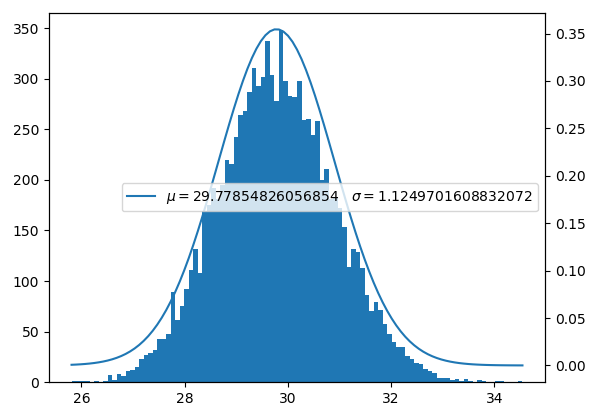
多元高斯分布的期望模长

import matplotlib.pyplot as plt
import numpy as np

n = 512
mus = np.random.random(n)*2-1
sigmas = np.random.random(n)*2
xs = np.array([np.random.normal(mu, sigma, (100000)) for mu, sigma in zip(mus, sigmas)]).T
feat_len = np.linalg.norm(xs, axis=1)
print(feat_len.shape)

mean_feat_len = np.mean(feat_len)
sigma_feat_len = np.std(feat_len)


def gauss(xs, mu, sigma):
    return 1 / (sigma * (2 * np.pi) ** 0.5) * np.exp(-(xs - mu) ** 2 / (2 * sigma ** 2))


_, edges, _ = plt.hist(feat_len, 100)
ax = plt.twinx()
ax.plot(edges, gauss(edges, mean_feat_len, sigma_feat_len), label="$mu=%squad sigma=%s$" % (mean_feat_len, sigma_feat_len))
plt.legend()
my_mu = np.sum(mus ** 2 + sigmas ** 2) ** 0.5
my_sigma = np.mean(sigmas ** 2) ** 0.5
print("my_mu", my_mu, "my_sigma", my_sigma)
plt.show() 

从此实验可以看出，高维空间中样本到原点的距离几乎都相等，mu很大，sigma却很小，同时样本的模长满足正态分布。
不仅仅相对于原点，对于空间中的任何一个点，距离都满足高斯分布，并且mu很大，sigma却很小。这表明高维空间中99.97%的点到某个点的距离几乎相同。因此高维空间聚类的阈值可以设置为$ mu - 3sigma $
高维空间中从任意一个点向周围望去，会发现大多数点离自己都很远很远，每个人都感觉到自己是宇宙的中心，感觉其它点像是分布在球壳上，而自己则处于球心，因为其它点到自己的距离几乎是相等的。

import matplotlib.pyplot as plt
import numpy as np

n = 512
mus = np.random.random(n) * 2 - 1
sigmas = np.random.random(n) * 2
xs = np.array([np.random.normal(mu, sigma, (10000)) for mu, sigma in zip(mus, sigmas)]).T


def gauss(xs, mu, sigma):
    return 1 / (sigma * (2 * np.pi) ** 0.5) * np.exp(-(xs - mu) ** 2 / (2 * sigma ** 2))


def show(feat_len):
    mean_feat_len = np.mean(feat_len)
    sigma_feat_len = np.std(feat_len)
    _, edges, _ = plt.hist(feat_len, 100)
    ax = plt.twinx()
    ax.plot(edges, gauss(edges, mean_feat_len, sigma_feat_len), label="$mu=%squad sigma=%s$" % (mean_feat_len, sigma_feat_len))
    plt.legend()
    plt.show()


feat_len = np.linalg.norm(xs, axis=1)
my_mu = np.sum(mus ** 2 + sigmas ** 2) ** 0.5
my_sigma = np.mean(sigmas ** 2) ** 0.5
print("my_mu", my_mu, "my_sigma", my_sigma)
print(feat_len.shape)
show(feat_len)
for i in range(10):
    show(np.linalg.norm(xs - xs[i], axis=1))

这个图横轴表示地球半径，纵轴表示该层分布的生物数量，会发现大部分生物都集中在了地壳上，低维空间中几乎不存在。

高维球体

高维球体

高维空间的特点

每个点从自身看去，会发现自己周围朋友很少，自己很孤独，大部分点离自己很遥远，这是每个点的特征。

为什么会出现这种情况呢？低维空间中，每一维度的尺度占整体距离的比例比较大，没一个维度都显得举足轻重。高维空间中，每个维度对于整体距离的贡献是近似的。点靠近球心的概率非常低。比如512维空间中，要想靠近原点，那就要做到512次全部都是0，这是非常难的一件事，因此没有点会靠近原点。在高维空间中，每个点到原点的距离都有一种趋同的趋势。也就是说，在高维空间中，人人平等。

每维都是均匀分布，距离如何分布

即便每维都是均匀分布，最终距离也是正态分布。正态分布无所不在。
这就是大数定理：N个独立同分布的样本，它们的某种统计量呈现正态分布。
随着维度的上升，sigma占mu的比例越来越小。

import matplotlib.pyplot as plt
import numpy as np

n = 102
min_value = np.random.random(n) * 2 - 10
max_value = np.random.random(n) * 2 + 15
xs = np.array([np.random.uniform(mi, ma, (10000)) for mi, ma in zip(min_value, max_value)]).T


def gauss(xs, mu, sigma):
    return 1 / (sigma * (2 * np.pi) ** 0.5) * np.exp(-(xs - mu) ** 2 / (2 * sigma ** 2))


def show(feat_len):
    mean_feat_len = np.mean(feat_len)
    sigma_feat_len = np.std(feat_len)
    center_count = np.argwhere(feat_len < mean_feat_len - 3 * sigma_feat_len).__len__() + np.argwhere(feat_len > mean_feat_len + 3 * sigma_feat_len).__len__()
    _, edges, _ = plt.hist(feat_len, 100)
    ax = plt.twinx()
    ax.plot(edges, gauss(edges, mean_feat_len, sigma_feat_len), label="$mu=%squad sigma=%s quad ratio=%s$" % (mean_feat_len, sigma_feat_len, center_count / len(feat_len) * 100))
    plt.legend()
    plt.show()


feat_len = np.linalg.norm(xs, axis=1)
print(feat_len.shape)
show(feat_len)
for i in range(10):
    show(np.linalg.norm(xs - xs[i], axis=1))

使用余弦距离也能看见高斯分布

在高维空间中，使用余弦距离比使用欧氏距离要好得多，因为欧氏距离太陡峭了（mu很大，sigma很小，造成正态分布的曲线非常陡峭）。

import matplotlib.pyplot as plt
import numpy as np

n = 512
min_value = np.random.random(n) * 2 - 10
max_value = np.random.random(n) * 2 + 15
xs = np.array([np.random.uniform(mi, ma, (10000)) for mi, ma in zip(min_value, max_value)]).T


def gauss(xs, mu, sigma):
    return 1 / (sigma * (2 * np.pi) ** 0.5) * np.exp(-(xs - mu) ** 2 / (2 * sigma ** 2))


def show(feat_len):
    mean_feat_len = np.mean(feat_len)
    sigma_feat_len = np.std(feat_len)
    _, edges, _ = plt.hist(feat_len, 100)
    ax = plt.twinx()
    ax.plot(edges, gauss(edges, mean_feat_len, sigma_feat_len), label="$mu=%squad sigma=%s$" % (mean_feat_len, sigma_feat_len))
    plt.legend()
    plt.show()


for i in range(10):
    angle = xs[np.random.randint(0, len(xs))]
    feat_len = np.dot(xs, angle) / np.linalg.norm(xs, axis=1)
    show(feat_len)

原因

对于随机向量而言，随着维度的增加，各维的均值是累积的，而方差会互相抵消从而导致方差无法累积，这就导致高维空间中方差占均值的比例越来越小，于是所有点到某个点的距离都趋近相同了。
均值可以累积，方差互相抵消不可累积，这就是为啥数据量多了之后，样本的某种范数趋近于正态分布。

高尔顿钉板

高斯分布为何如此常见？它是怎样形成的？

中心极限定理的本质是什么？

弗朗西斯·高尔顿爵士（1822－1911），查尔斯·达尔文的表弟，英格兰维多利亚时代的博学家、人类学家、优生学家、热带探险家、地理学家、发明家、气象学家、统计学家、心理学家和遗传学家。

他发明了一个叫做高尔顿钉板的装置，展示了正态分布的产生过程：高尔顿钉板是一种装置，它是一个木盒子，里面均匀分布着若干排钉子。从入口处把小球倒入钉板，最终箱子里面形成的分布近似为高斯分布。弹珠往下滚的时候，撞到钉子就会随机选择往左边走，还是往右边走。一颗弹珠一路滚下来会多次选择方向，最终的分布会接近正态分布。
高尔顿钉板有两处细节：

• 顶上只有一处开口：这是要求弹珠的起始状态一致。类比女性身高的例子，就是要求至少物种一致，总不能猪和人一起比较。换成数学用语就是要求同分布。
• 开口位于顶部中央：这倒无所谓，开在别的位置，分布形态不变，只是平移

import matplotlib.pyplot as plt
import numpy as np

n = 100000  # 小球的个数
box_width = 1  # 箱子的宽度
row_count = 1000  # 每行钉子的个数
col_count = 1000  # 每列钉子的个数

a = np.ones(n) * box_width / 2  # 开始时的位置
for i in range(row_count):
    delta = (np.random.randint(0, 2, n) - 0.5) * box_width / col_count
    a += delta
    a = np.clip(a, 0, box_width)
plt.hist(a, col_count // 2)
plt.show()

高尔顿钉板可以做许多变动，变动之后依然是高斯分布。如：

• 移动开口的水平位置
• 改变小球碰到钉子之后的随机性，即便是不均匀的分布最终也会形成高斯分布

import matplotlib.pyplot as plt
import numpy as np

n = 50000  # 小球的个数
box_width = 1  # 箱子的宽度
row_count = 1000  # 每行钉子的个数
col_count = 1000  # 每列钉子的个数

a = np.ones(n) * box_width / 2  # 开始时的位置
for i in range(row_count):
    delta = ((np.random.randint(0, 13, n)) - 6.5) / 6.5 * box_width / col_count
    a += delta
    a = np.clip(a, 0, box_width)
plt.hist(a, col_count // 4)
plt.show()

让小球总是往右边跑

import matplotlib.pyplot as plt
import numpy as np

n = 50000  # 小球的个数
box_width = 1  # 箱子的宽度
row_count = 1000  # 每行钉子的个数
col_count = 1000  # 每列钉子的个数

a = np.ones(n) * box_width / 2  # 开始时的位置
for i in range(row_count):
    delta = ((np.random.randint(0, 13, n))) / 13 * box_width / col_count
    a += delta
    a = np.clip(a, 0, box_width)
plt.hist(a, col_count // 4)
plt.show()

自然界中为何如此多的变量都服从高斯分布？因为每个变量都是由一系列随机变量组成的。例如人的身高由饮食、气候、基因等很多独立随机变量组成，这些独立随机变量就像钉子一样一层一层地摆放，最初人的身高是固定的（就像从中间扔下来的小球），经过这么多随机因素之后人的身高就变成了正态分布。
中心极限定理：大量独立同分布的变量（每个变量都相当于一次采样）最终形成的分布是高斯分布。

高斯分布凭啥凌驾于其它任意分布之上？
高斯分布是一种毫无道理的分布，它只是一种拟合，这种拟合非常逼真，于是才得到广泛应用。

参考资料

高斯分布为何如此常见