一、外极几何
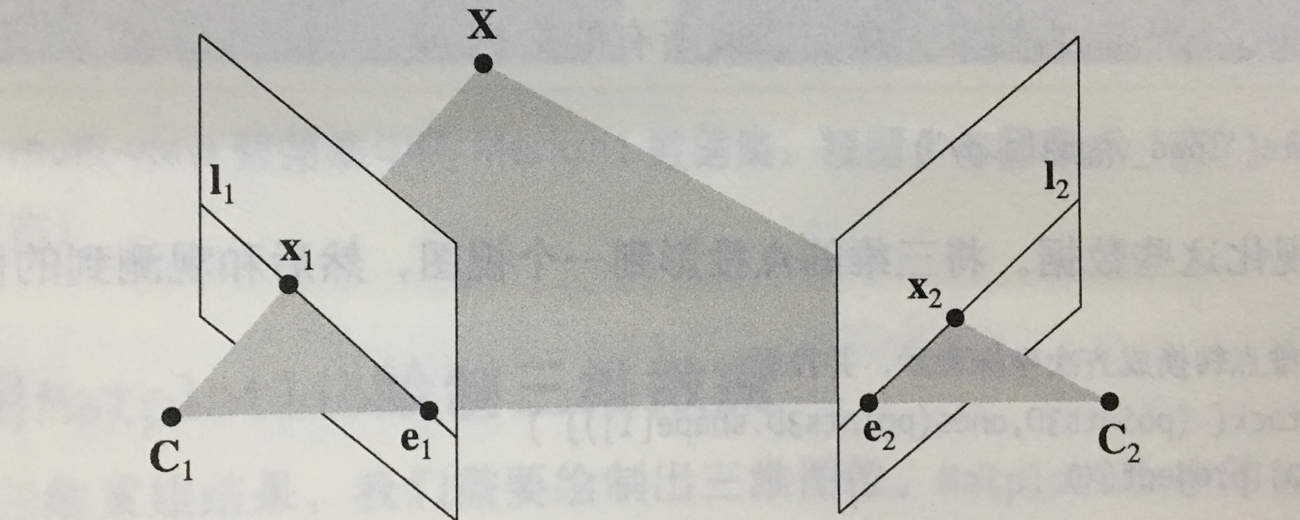
图一:外极几何示意图:
在这两个视图中,分别将三维点X投影为x1和x2.两个相机中心之间的基线C1和C2与图像平面相交于外极点e1和e2,线I1和I2成为外极线。
如果已经知道相机的参数,那么在重建过程中遇到的问题就是两幅图像之间的关系,外极线约束的主要作用就是限制对应特征点的搜索范围,将对应特征点的搜索限制在极线上。
二、基础矩阵
1.基础矩阵概述:
1)两幅图像之间的约束关系使用代数的方式表示出来即为基本矩阵。
2)基础矩阵F满足:![]()
3)基础矩阵可以用于简化匹配和去除错配特征
2.八点算法估算基础矩阵F
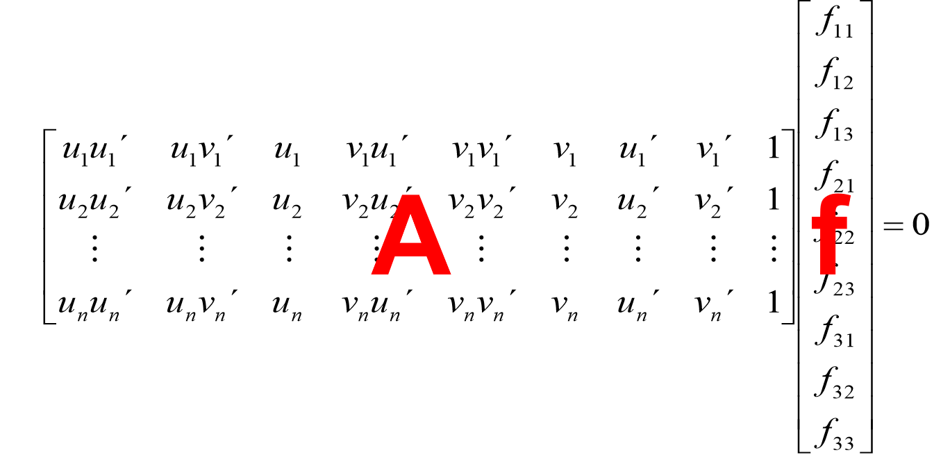
1)原理:任给两幅图像中的匹配点 x 与 x’ ,令 x=(u,v,1)^T ,x’=(u’,v’,1)^T
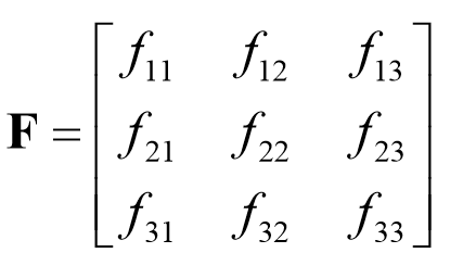
基础矩阵F是一个3×3的秩为2的矩阵,一般记基础矩阵F为:
有相应方程:
![]()
由矩阵乘法可知有:
2)优点: 线性求解,容易实现,运行速度快 。
缺点:对噪声敏感。
三、照相机和三维结构的计算
1.三角剖分
给定照相机参数模型,图像点可以通过三角剖分来恢复出这些点的三维位置。

得到基础矩阵:

通过三角剖分得到的特征点:估计点和实际图像点很接近,可以很好地匹配。

三角剖分后有36个特征匹配的点:
照相机矩阵
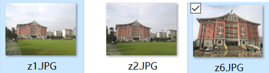
1)数据集:
2)实验结果
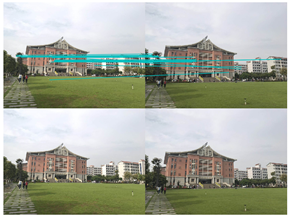
a.sift特征匹配结果:

b.处理过后:
z1.jpg和z2.jpg:
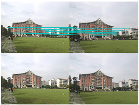
z1.jpg和z6.jpg:
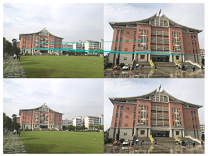
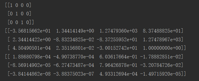
c.由三维点得到照相机矩阵
图z1的照相机矩阵

图z2的照相机矩阵
图z6的照相机矩阵
(二)室内
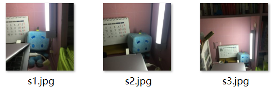
1.数据集:
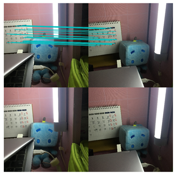
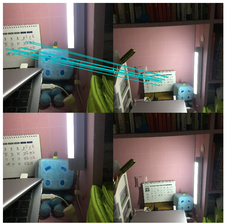
2.s1与s2进行sift特征匹配:有180个特征匹配点
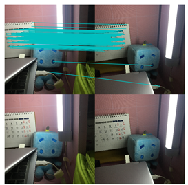
2.s1与s2通过三角剖分得到的特征点:估计点和实际图像点很接近,可以很好地匹配。
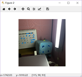
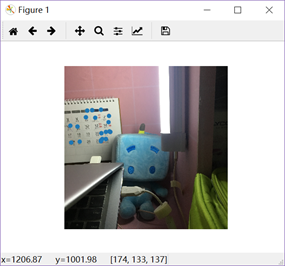
3.三角剖分后有29个特征匹配的点:
4.s1和拍摄距离较远的图片s3进行特征匹配
.
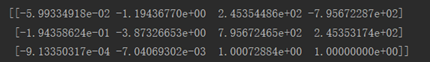
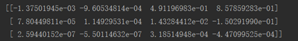
5.由三维点得到三张图的照相机矩阵(顺序:s1,s2,s3)
四、实验中遇到的问题
头文件问题:将头文件改为


 1 # In[1]:
 2 from PIL import Image
 3 from numpy import *
 4 from pylab import *
 5 import numpy as np
 6 from imp import reload
 7 # In[2]:
 8
 9 from PCV.geometry import camera
10 from PCV.geometry import homography
11 from PCV.geometry import sfm
12 from PCV.localdescriptors import sift
五、参考文献
三角剖分算法(delaunay) https://blog.csdn.net/aaronmorgan/article/details/80389142
三维重建(一)外极几何,基础矩阵及求解https://blog.csdn.net/lhanchao/article/details/51834223
六、附代码
  1 #!/usr/bin/env python
  2 # coding: utf-8
  3
  4 # In[1]:
  5 from PIL import Image
  6 from numpy import *
  7 from pylab import *
  8 import numpy as np
  9 from imp import reload
 10 # In[2]:
 11
 12 from PCV.geometry import camera
 13 from PCV.geometry import homography
 14 from PCV.geometry import sfm
 15 from PCV.localdescriptors import sift
 16
 17 camera = reload(camera)
 18 homography = reload(homography)
 19 sfm = reload(sfm)
 20 sift = reload(sift)
 21
 22
 23 # In[3]:
 24
 25
 26 # Read features
 27 im1 = array(Image.open('D:/there/pictures/s1.JPG'))
 28 sift.process_image('D:/there/pictures/s1.JPG', 'im1.sift')
 29 l1, d1 = sift.read_features_from_file('im1.sift')
 30
 31 im2 = array(Image.open('D:/there/pictures/s2.JPG'))
 32 sift.process_image('D:/there/pictures/s2.JPG', 'im2.sift')
 33 l2, d2 = sift.read_features_from_file('im2.sift')
 34
 35
 36 # In[9]:
 37
 38
 39 matches = sift.match_twosided(d1, d2)
 40
 41
 42 # In[10]:
 43
 44
 45 ndx = matches.nonzero()[0]
 46 x1 = homography.make_homog(l1[ndx, :2].T)
 47 ndx2 = [int(matches[i]) for i in ndx]
 48 x2 = homography.make_homog(l2[ndx2, :2].T)
 49
 50 x1n = x1.copy()
 51 x2n = x2.copy()
 52
 53
 54 # In[11]:
 55
 56
 57 print(len(ndx))
 58
 59
 60 # In[12]:
 61
 62
 63 figure(figsize=(16,16))
 64 sift.plot_matches(im1, im2, l1, l2, matches, True)
 65 show()
 66
 67
 68 # In[13]:
 69
 70
 71 # Chapter 5 Exercise 1
 72 # Don't use K1, and K2
 73
 74 #def F_from_ransac(x1, x2, model, maxiter=5000, match_threshold=1e-6):
 75 def F_from_ransac(x1, x2, model, maxiter=5000, match_threshold=1e-6):
 76     """ Robust estimation of a fundamental matrix F from point
 77     correspondences using RANSAC (ransac.py from
 78     http://www.scipy.org/Cookbook/RANSAC).
 79
 80     input: x1, x2 (3*n arrays) points in hom. coordinates. """
 81
 82     from PCV.tools import ransac
 83     data = np.vstack((x1, x2))
 84     d = 20 # 20 is the original
 85     # compute F and return with inlier index
 86     F, ransac_data = ransac.ransac(data.T, model,
 87                                    8, maxiter, match_threshold, d, return_all=True)
 88     return F, ransac_data['inliers']
 89
 90
 91 # In[15]:
 92
 93
 94 # find E through RANSAC
 95 model = sfm.RansacModel()
 96 F, inliers = F_from_ransac(x1n, x2n, model, maxiter=5000, match_threshold=1e-3)
 97
 98
 99 # In[16]:
100
101
102 print (len(x1n[0]))
103 print (len(inliers))
104
105
106 # In[17]:
107
108
109 P1 = array([[1, 0, 0, 0], [0, 1, 0, 0], [0, 0, 1, 0]])
110 P2 = sfm.compute_P_from_fundamental(F)
111
112
113 # In[18]:
114
115
116 # triangulate inliers and remove points not in front of both cameras
117 X = sfm.triangulate(x1n[:, inliers], x2n[:, inliers], P1, P2)
118
119
120 # In[19]:
121
122
123 # plot the projection of X
124 cam1 = camera.Camera(P1)
125 cam2 = camera.Camera(P2)
126 x1p = cam1.project(X)
127 x2p = cam2.project(X)
128
129
130 # In[20]:
131
132
133 figure()
134 imshow(im1)
135 gray()
136 plot(x1p[0], x1p[1], 'o')
137 #plot(x1[0], x1[1], 'r.')
138 axis('off')
139
140 figure()
141 imshow(im2)
142 gray()
143 plot(x2p[0], x2p[1], 'o')
144 #plot(x2[0], x2[1], 'r.')
145 axis('off')
146 show()
147
148
149 # In[21]:
150
151
152 figure(figsize=(16, 16))
153 im3 = sift.appendimages(im1, im2)
154 im3 = vstack((im3, im3))
155
156 imshow(im3)
157
158 cols1 = im1.shape[1]
159 rows1 = im1.shape[0]
160 for i in range(len(x1p[0])):
161     if (0<= x1p[0][i]<cols1) and (0<= x2p[0][i]<cols1) and (0<=x1p[1][i]<rows1) and (0<=x2p[1][i]<rows1):
162         plot([x1p[0][i], x2p[0][i]+cols1],[x1p[1][i], x2p[1][i]],'c')
163 axis('off')
164 show()
165
166
167 # In[22]:
168
169
170 print (F)
171
172
173 # In[23]:
174
175
176 # Chapter 5 Exercise 2
177
178 x1e = []
179 x2e = []
180 ers = []
181 for i,m in enumerate(matches):
182     if m>0: #plot([locs1[i][0],locs2[m][0]+cols1],[locs1[i][1],locs2[m][1]],'c')
183         p1 = array([l1[i][0], l1[i][1], 1])
184         p2 = array([l2[m][0], l2[m][1], 1])
185         # Use Sampson distance as error
186         Fx1 = dot(F, p1)
187         Fx2 = dot(F, p2)
188         denom = Fx1[0]**2 + Fx1[1]**2 + Fx2[0]**2 + Fx2[1]**2
189         e = (dot(p1.T, dot(F, p2)))**2 / denom
190         x1e.append([p1[0], p1[1]])
191         x2e.append([p2[0], p2[1]])
192         ers.append(e)
193 x1e = array(x1e)
194 x2e = array(x2e)
195 ers = array(ers)
196
197
198 # In[24]:
199
200
201 indices = np.argsort(ers)
202 x1s = x1e[indices]
203 x2s = x2e[indices]
204 ers = ers[indices]
205 x1s = x1s[:20]
206 x2s = x2s[:20]
207
208
209 # In[25]:
210
211
212 figure(figsize=(16, 16))
213 im3 = sift.appendimages(im1, im2)
214 im3 = vstack((im3, im3))
215
216 imshow(im3)
217
218 cols1 = im1.shape[1]
219 rows1 = im1.shape[0]
220 for i in range(len(x1s)):
221     if (0<= x1s[i][0]<cols1) and (0<= x2s[i][0]<cols1) and (0<=x1s[i][1]<rows1) and (0<=x2s[i][1]<rows1):
222         plot([x1s[i][0], x2s[i][0]+cols1],[x1s[i][1], x2s[i][1]],'c')
223 axis('off')
224 show()
225
226
227 # In[ ]:
  1 #!/usr/bin/env python
  2 # coding: utf-8
  3
  4 # In[1]:
  5
  6 from PIL import Image
  7 from numpy import *
  8 from pylab import *
  9 import numpy as np
 10 from imp import reload
 11
 12
 13 # In[2]:
 14
 15
 16 from PCV.geometry import camera
 17 from PCV.geometry import homography
 18 from PCV.geometry import sfm
 19 from PCV.localdescriptors import sift
 20
 21 camera = reload(camera)
 22 homography = reload(homography)
 23 sfm = reload(sfm)
 24 sift = reload(sift)
 25
 26
 27 # In[3]:
 28
 29
 30 # Read features
 31 im1 = array(Image.open('D:/there/pictures/s1.JPG'))
 32 sift.process_image('D:/there/pictures/s1.JPG', 'im1.sift')
 33
 34 im2 = array(Image.open('D:/there/pictures/s2.JPG'))
 35 sift.process_image('D:/there/pictures/s2.JPG', 'im2.sift')
 36
 37
 38 # In[4]:
 39
 40
 41 l1, d1 = sift.read_features_from_file('im1.sift')
 42 l2, d2 = sift.read_features_from_file('im2.sift')
 43
 44
 45 # In[5]:
 46
 47
 48 matches = sift.match_twosided(d1, d2)
 49
 50
 51 # In[6]:
 52
 53
 54 ndx = matches.nonzero()[0]
 55 x1 = homography.make_homog(l1[ndx, :2].T)
 56 ndx2 = [int(matches[i]) for i in ndx]
 57 x2 = homography.make_homog(l2[ndx2, :2].T)
 58
 59 d1n = d1[ndx]
 60 d2n = d2[ndx2]
 61 x1n = x1.copy()
 62 x2n = x2.copy()
 63
 64
 65 # In[7]:
 66
 67
 68 figure(figsize=(16,16))
 69 sift.plot_matches(im1, im2, l1, l2, matches, True)
 70 show()
 71
 72
 73 # In[26]:
 74
 75
 76 #def F_from_ransac(x1, x2, model, maxiter=5000, match_threshold=1e-6):
 77 def F_from_ransac(x1, x2, model, maxiter=5000, match_threshold=1e-6):
 78     """ Robust estimation of a fundamental matrix F from point
 79     correspondences using RANSAC (ransac.py from
 80     http://www.scipy.org/Cookbook/RANSAC).
 81
 82     input: x1, x2 (3*n arrays) points in hom. coordinates. """
 83
 84     from PCV.tools import ransac
 85     data = np.vstack((x1, x2))
 86     d = 10 # 20 is the original
 87     # compute F and return with inlier index
 88     F, ransac_data = ransac.ransac(data.T, model,
 89                                    8, maxiter, match_threshold, d, return_all=True)
 90     return F, ransac_data['inliers']
 91
 92
 93 # In[27]:
 94
 95
 96 # find F through RANSAC
 97 model = sfm.RansacModel()
 98 F, inliers = F_from_ransac(x1n, x2n, model, maxiter=5000, match_threshold=1e-1)
 99 print (F)
100
101
102 # In[28]:
103
104
105 P1 = array([[1, 0, 0, 0], [0, 1, 0, 0], [0, 0, 1, 0]])
106 P2 = sfm.compute_P_from_fundamental(F)
107
108
109 # In[29]:
110
111
112 print (P2)
113 print (F)
114
115
116 # In[30]:
117
118
119 # P2, F (1e-4, d=20)
120 # [[ -1.48067422e+00   1.14802177e+01   5.62878044e+02   4.74418238e+03]
121 #  [  1.24802182e+01  -9.67640761e+01  -4.74418113e+03   5.62856097e+02]
122 #  [  2.16588305e-02   3.69220292e-03  -1.04831621e+02   1.00000000e+00]]
123 # [[ -1.14890281e-07   4.55171451e-06  -2.63063628e-03]
124 #  [ -1.26569570e-06   6.28095242e-07   2.03963649e-02]
125 #  [  1.25746499e-03  -2.19476910e-02   1.00000000e+00]]
126
127
128 # In[31]:
129
130
131 # triangulate inliers and remove points not in front of both cameras
132 X = sfm.triangulate(x1n[:, inliers], x2n[:, inliers], P1, P2)
133
134
135 # In[32]:
136
137
138 # plot the projection of X
139 cam1 = camera.Camera(P1)
140 cam2 = camera.Camera(P2)
141 x1p = cam1.project(X)
142 x2p = cam2.project(X)
143
144
145 # In[33]:
146
147
148 figure(figsize=(16, 16))
149 imj = sift.appendimages(im1, im2)
150 imj = vstack((imj, imj))
151
152 imshow(imj)
153
154 cols1 = im1.shape[1]
155 rows1 = im1.shape[0]
156 for i in range(len(x1p[0])):
157     if (0<= x1p[0][i]<cols1) and (0<= x2p[0][i]<cols1) and (0<=x1p[1][i]<rows1) and (0<=x2p[1][i]<rows1):
158         plot([x1p[0][i], x2p[0][i]+cols1],[x1p[1][i], x2p[1][i]],'c')
159 axis('off')
160 show()
161
162
163 # In[34]:
164
165
166 d1p = d1n[inliers]
167 d2p = d2n[inliers]
168
169
170 # In[35]:
171
172
173 # Read features
174 im3 = array(Image.open('D:/there/pictures/s3.JPG'))
175 sift.process_image('D:/there/pictures/s3.JPG', 'im3.sift')
176 l3, d3 = sift.read_features_from_file('im3.sift')
177
178
179 # In[36]:
180
181
182 matches13 = sift.match_twosided(d1p, d3)
183
184
185 # In[37]:
186
187
188 ndx_13 = matches13.nonzero()[0]
189 x1_13 = homography.make_homog(x1p[:, ndx_13])
190 ndx2_13 = [int(matches13[i]) for i in ndx_13]
191 x3_13 = homography.make_homog(l3[ndx2_13, :2].T)
192
193
194 # In[38]:
195
196
197 figure(figsize=(16, 16))
198 imj = sift.appendimages(im1, im3)
199 imj = vstack((imj, imj))
200
201 imshow(imj)
202
203 cols1 = im1.shape[1]
204 rows1 = im1.shape[0]
205 for i in range(len(x1_13[0])):
206     if (0<= x1_13[0][i]<cols1) and (0<= x3_13[0][i]<cols1) and (0<=x1_13[1][i]<rows1) and (0<=x3_13[1][i]<rows1):
207         plot([x1_13[0][i], x3_13[0][i]+cols1],[x1_13[1][i], x3_13[1][i]],'c')
208 axis('off')
209 show()
210
211
212 # In[39]:
213
214
215 P3 = sfm.compute_P(x3_13, X[:, ndx_13])
216
217
218 # In[40]:
219
220
221 print (P3)
222
223
224 # In[41]:
225
226
227 print (P1)
228 print (P2)
229 print (P3)
230
231
232 # In[22]:
233
234
235 # Can't tell the camera position because there's no calibration matrix (K)