花纹的生成可以使用贴图的方式,同样也可以使用方程,本文列出了几种常用曲线的方程式,以取代贴图方式完成特定花纹的生成。
注意极坐标的使用.................
前面部分基础资料,参考:Python:Matplotlib 画曲线和柱状图(Code)
Pyplot教程:https://matplotlib.org/gallery/index.html#pyplots-examples

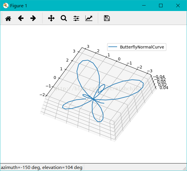
顾名思义,蝴蝶曲线(Butterfly curve )就是曲线形状如同蝴蝶。蝴蝶曲线如图所示,以方程描述,是一条六次平面曲线。如果大家觉得这个太过简单,别着急,还有第二种。如图所示,以方程描述,这是一个极坐标方程。通过改变这个方程中的变量θ,可以得到不同形状与方向的蝴蝶曲线。如果再施以复杂的组合和变换,我们看到的就完全称得上是一幅艺术品了。
Python代码:
import numpy as np
import matplotlib.pyplot as plt
import os,sys,caffe
import matplotlib as mpl
from mpl_toolkits.mplot3d import Axes3D #draw lorenz attractor
# %matplotlib inline
from math import sin, cos, pi
import math
def mainex():
#drawSpringCrurve();#画柱坐标系螺旋曲线
#HelicalCurve();#采用柱坐标系#尖螺旋曲线
#Votex3D();
#phoenixCurve();
#ButterflyCurve();
#ButterflyNormalCurve();
#dicareCurve2d();
#WindmillCurve3d();
#HelixBallCurve();#球面螺旋线
#AppleCurve();
#HelixInCircleCurve();#使用scatter,排序有问题
seperialHelix();
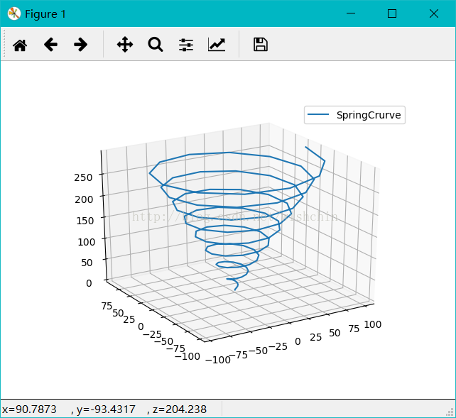
def drawSpringCrurve():
#碟形弹簧
#圓柱坐标
#方程:
#import matplotlib as mpl
#from mpl_toolkits.mplot3d import Axes3D
#import numpy as np
#import matplotlib.pyplot as plt
mpl.rcParams['legend.fontsize'] = 10;
fig = plt.figure();
ax = fig.gca(projection='3d');
# Prepare arrays x, y, z
#theta = np.linspace(-4 * np.pi, 4 * np.pi, 100)
#z = np.linspace(-2, 2, 100)
#r = z**2 + 1
t = np.arange(0,100,1);
r = t*0 +20;
theta = t*3600 ;
z = np.arange(0,100,1);
for i in range(100):
z[i] =(sin(3.5*theta[i]-90))+24*t[i];
x = r * np.sin(theta);
y = r * np.cos(theta);
ax.plot(x, y, z, label='SpringCrurve');
ax.legend();
plt.show();
def HelicalCurve():
#螺旋曲线#采用柱坐标系
t = np.arange(0,100,1);
r =t ;
theta=10+t*(20*360);
z =t*3;
x = r * np.sin(theta);
y = r * np.cos(theta);
mpl.rcParams['legend.fontsize'] = 10;
fig = plt.figure();
ax = fig.gca(projection='3d');
ax.plot(x, y, z, label='HelicalCurve');
ax.legend();
plt.show();
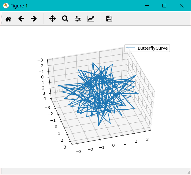
def ButterflyCurve():
#蝶形曲线,使用球坐标系#或许公式是错误的,应该有更加复杂的公式
t = np.arange(0,4,0.01);
r = 8 * t;
theta = 3.6 * t * 2*1 ;
phi = -3.6 * t * 4*1;
x = t*1;
y = t*1;
#z = t*1;
z =0
for i in range(len(t)):
x[i] = r[i] * np.sin(theta[i])*np.cos(phi[i]);
y[i] = r[i] * np.sin(theta[i])*np.sin(phi[i]);
#z[i] = r[i] * np.cos(theta[i]);
mpl.rcParams['legend.fontsize'] = 10;
fig = plt.figure();
ax = fig.gca(projection='3d');
ax.plot(x, y, z, label='ButterflyCurve');
#ax.scatter(x, y, z, label='ButterflyCurve');
ax.legend();
plt.show();
def ButterflyNormalCurve():
#蝶形曲线,使用球坐标系#或许公式是错误的,应该有更加复杂的公式
#螺旋曲线#采用柱坐标系
#t = np.arange(0,100,1);
theta=np.arange(0,6,0.1);#(0,72,0.1);
r =theta*0;
z =theta*0;
x =theta*0;
y =theta*0;
for i in range(len(theta)):
r[i] = np.power(math.e,sin(theta[i]))- 2*cos(4*theta[i])
+ np.power( sin(1/24 * (2*theta[i] -pi ) ) , 5 );
#x[i] = r[i] * np.sin(theta[i]);
#y[i] = r[i] * np.cos(theta[i]);
x = r * np.sin(theta);
y = r * np.cos(theta);
mpl.rcParams['legend.fontsize'] = 10;
fig = plt.figure();
ax = fig.gca(projection='3d');
ax.plot(x, y, z, label='ButterflyNormalCurve');
ax.legend();
plt.show();
def phoenixCurve():
#蝶形曲线,使用球坐标系
t = np.arange(0,100,1);
r = 8 * t;
theta = 360 * t * 4 ;
phi = -360 * t * 8;
x = t*1;
y = t*1;
z = t*1;
for i in range(len(t)):
x[i] = r[i] * np.sin(theta[i])*np.cos(phi[i]);
y[i] = r[i] * np.sin(theta[i])*np.sin(phi[i]);
z[i] = r[i] * np.cos(theta[i]);
mpl.rcParams['legend.fontsize'] = 10;
fig = plt.figure();
ax = fig.gca(projection='3d');
ax.plot(x, y, z, label='phoenixCurve');
ax.legend();
plt.show();
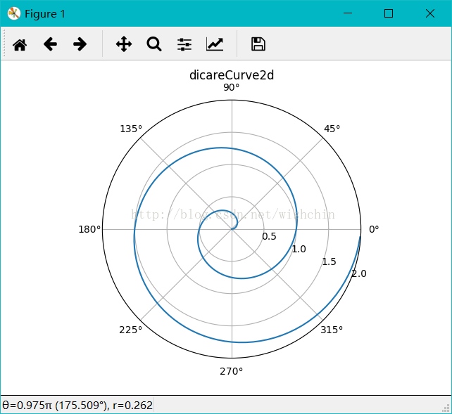
def dicareCurve2d():
r = np.arange(0, 2, 0.01)
theta = 2 * np.pi * r
ax = plt.subplot(111, projection='polar')
ax.plot(theta, r)
ax.set_rmax(2)
ax.set_rticks([0.5, 1, 1.5, 2]) # Less radial ticks
ax.set_rlabel_position(-22.5) # Move radial labels away from plotted line
ax.grid(True)
ax.set_title("dicareCurve2d", va='bottom')
plt.show();
def WindmillCurve3d():
#风车曲线
t = np.arange(0,2,0.01);
r =t*0+1 ;
#r=1
ang =36*t;#ang =360*t;
s =2*pi*r*t;
x = t*1;
y = t*1;
for i in range(len(t)):
x[i] = s[i]*cos(ang[i]) +s[i]*sin(ang[i]) ;
y[i] = s[i]*sin(ang[i]) -s[i]*cos(ang[i]) ;
z =t*0;
mpl.rcParams['legend.fontsize'] = 10;
fig = plt.figure();
ax = fig.gca(projection='3d');
ax.plot(x, y, z, label='WindmillCurve3d');
ax.legend();
plt.show();
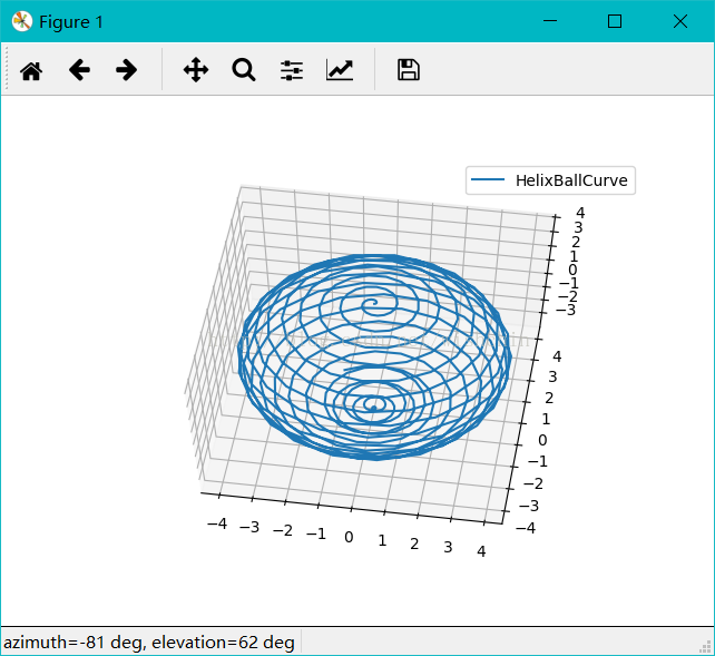
def HelixBallCurve():
#螺旋曲线,使用球坐标系
t = np.arange(0,2,0.005);
r =t*0+4 ;
theta =t*1.8
phi =t*3.6*20
x = t*1;
y = t*1;
z = t*1;
for i in range(len(t)):
x[i] = r[i] * np.sin(theta[i])*np.cos(phi[i]);
y[i] = r[i] * np.sin(theta[i])*np.sin(phi[i]);
z[i] = r[i] * np.cos(theta[i]);
mpl.rcParams['legend.fontsize'] = 10;
fig = plt.figure();
ax = fig.gca(projection='3d');
ax.plot(x, y, z, label='HelixBallCurve');
ax.legend();
plt.show();
def seperialHelix():
#螺旋曲线,使用球坐标系
t = np.arange(0,2,0.1);
n = np.arange(0,2,0.1);
r =t*0+4 ;
theta =n*1.8 ;
phi =n*3.6*20;
x = t*0;
y = t*0;
z = t*0;
for i in range(len(t)):
x[i] = r[i] * np.sin(theta[i])*np.cos(phi[i]);
y[i] = r[i] * np.sin(theta[i])*np.sin(phi[i]);
z[i] = r[i] * np.cos(theta[i]);
mpl.rcParams['legend.fontsize'] = 10;
fig = plt.figure();
ax = fig.gca(projection='3d');
ax.plot(x, y, z, label='ButterflyCurve');
ax.legend();
plt.show();
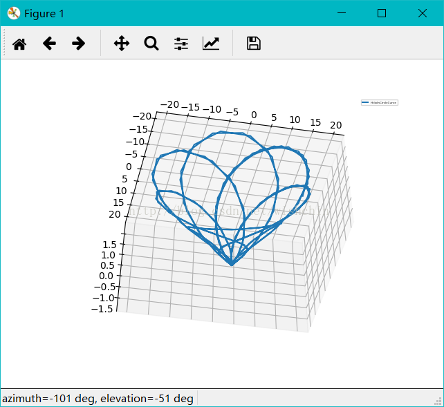
def AppleCurve():
#螺旋曲线
t = np.arange(0,2,0.01);
l=2.5
b=2.5
x = t*1;
y = t*1;
z =0;#z=t*0;
n = 36
for i in range(len(t)):
x[i]=3*b*cos(t[i]*n)+l*cos(3*t[i]*n)
y[i]=3*b*sin(t[i]*n)+l*sin(3*t[i]*n)
#x = r * np.sin(theta);
#y = r * np.cos(theta);
mpl.rcParams['legend.fontsize'] = 10;
fig = plt.figure();
ax = fig.gca(projection='3d');
ax.plot(x, y, z, label='AppleCurve');
ax.legend();
plt.show();
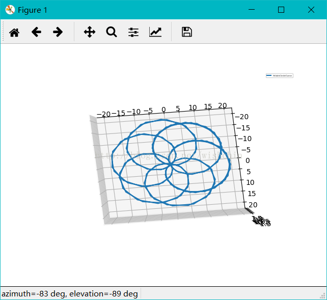
def HelixInCircleCurve():
#园内螺旋曲线#采用柱坐标系
t = np.arange(-1,1,0.01);
theta=t*36 ;#360 deta 0.005鸟巢网 #36 deta 0.005 圆内曲线
x = t*1;
y = t*1;
z = t*1;
r = t*1;
n = 1.2
for i in range(len(t)):
r[i]=10+10*sin(n*theta[i]);
z[i]=2*sin(n*theta[i]);
x[i] = r[i] * np.sin(theta[i]);
y[i] = r[i] * np.cos(theta[i]);
mpl.rcParams['legend.fontsize'] = 3;
fig = plt.figure();
ax = fig.gca(projection='3d');
ax.plot(x, y, z, label='HelixInCircleCurve');
#ax.scatter(x, y, z, label='HelixInCircleCurve');
ax.legend();
plt.show();
def Votex3D():
def midpoints(x):
sl = ()
for i in range(x.ndim):
x = (x[sl + np.index_exp[:-1]] + x[sl + np.index_exp[1:]]) / 2.0
sl += np.index_exp[:]
return x
# prepare some coordinates, and attach rgb values to each
r, g, b = np.indices((17, 17, 17)) / 16.0
rc = midpoints(r)
gc = midpoints(g)
bc = midpoints(b)
# define a sphere about [0.5, 0.5, 0.5]
sphere = (rc - 0.5)**2 + (gc - 0.5)**2 + (bc - 0.5)**2 < 0.5**2
# combine the color components
colors = np.zeros(sphere.shape + (3,))
colors[..., 0] = rc
colors[..., 1] = gc
colors[..., 2] = bc
# and plot everything
fig = plt.figure();
ax = fig.gca(projection='3d');
ax.voxels(r, g, b, sphere,
facecolors=colors,
edgecolors=np.clip(2*colors - 0.5, 0, 1), # brighter
linewidth=0.5);
ax.set(xlabel='r', ylabel='g', zlabel='b');
plt.show();
def drawFiveFlower():
theta=np.arange(0,2*np.pi,0.02)
#plt.subplot(121,polar=True)
#plt.plot(theta,2*np.ones_like(theta),lw=2)
#plt.plot(theta,theta/6,'--',lw=2)
#plt.subplot(122,polar=True)
plt.subplot(111,polar=True)
plt.plot(theta,np.cos(5*theta),'--',lw=2)
plt.plot(theta,2*np.cos(4*theta),lw=2)
plt.rgrids(np.arange(0.5,2,0.5),angle=45)
plt.thetagrids([0,45,90]);
plt.show();
if __name__ == '__main__':
import argparse
mainex();画图结果: