数据竞赛实战（1）——足球运动员身价估计

前言

1，背景介绍

　　每个足球运动员在转会市场都有各自的价码。本次数据练习的目的是根据球员的各项信息和能力来预测该球员的市场价值。

2，数据来源

　　FIFA2018

3，数据文件说明

　　数据文件分为三个：

train.csv 　　　　　 　 训练集  　 　 文件大小为2.20MB

test.csv          　　　　 预测集   　　 文件大小为1.44KB

sample_submit.csv 　  提交示例        文件大小为65KB

　　训练集共有10441条样本，预测集中有7000条样本。每条样本代表一位球员，数据中每个球员

有61项属性。数据中含有缺失值。

4，数据变量说明

id	行编号，没有实际意义
club	该球员所属的俱乐部。该信息已经被编码。
league	该球员所在的联赛。已被编码。
birth_date	生日。格式为月/日/年。
height_cm	身高（厘米）
weight_kg	体重（公斤）
nationality	国籍。已被编码。
potential	球员的潜力。数值变量。
pac	球员速度。数值变量。
sho	射门（能力值）。数值变量。
pas	传球（能力值）。数值变量。
dri	带球（能力值）。数值变量。
def	防守（能力值）。数值变量。
phy	身体对抗（能力值）。数值变量。
international_reputation	国际知名度。数值变量。
skill_moves	技巧动作。数值变量。
weak_foot	非惯用脚的能力值。数值变量。
work_rate_att	球员进攻的倾向。分类变量，Low, Medium, High。
work_rate_def	球员防守的倾向。分类变量，Low, Medium, High。
preferred_foot	惯用脚。1表示右脚、2表示左脚。
crossing	传中（能力值）。数值变量。
finishing	完成射门（能力值）。数值变量。
heading_accuracy	头球精度（能力值）。数值变量。
short_passing	短传（能力值）。数值变量。
volleys	凌空球（能力值）。数值变量。
dribbling	盘带（能力值）。数值变量。
curve	弧线（能力值）。数值变量。
free_kick_accuracy	定位球精度（能力值）。数值变量。
long_passing	长传（能力值）。数值变量。
ball_control	控球（能力值）。数值变量。
acceleration	加速度（能力值）。数值变量。
sprint_speed	冲刺速度（能力值）。数值变量。
agility	灵活性（能力值）。数值变量。
reactions	反应（能力值）。数值变量。
balance	身体协调（能力值）。数值变量。
shot_power	射门力量（能力值）。数值变量。
jumping	弹跳（能力值）。数值变量。
stamina	体能（能力值）。数值变量。
strength	力量（能力值）。数值变量。
long_shots	远射（能力值）。数值变量。
aggression	侵略性（能力值）。数值变量。
interceptions	拦截（能力值）。数值变量。
positioning	位置感（能力值）。数值变量。
vision	视野（能力值）。数值变量。
penalties	罚点球（能力值）。数值变量。
marking	卡位（能力值）。数值变量。
standing_tackle	断球（能力值）。数值变量。
sliding_tackle	铲球（能力值）。数值变量。
gk_diving	门将扑救（能力值）。数值变量。
gk_handling	门将控球（能力值）。数值变量。
gk_kicking	门将开球（能力值）。数值变量。
gk_positioning	门将位置感（能力值）。数值变量。
gk_reflexes	门将反应（能力值）。数值变量。
rw	球员在右边锋位置的能力值。数值变量。
rb	球员在右后卫位置的能力值。数值变量。
st	球员在射手位置的能力值。数值变量。
lw	球员在左边锋位置的能力值。数值变量。
cf	球员在锋线位置的能力值。数值变量。
cam	球员在前腰位置的能力值。数值变量。
cm	球员在中场位置的能力值。数值变量。
cdm	球员在后腰位置的能力值。数值变量。
cb	球员在中后卫的能力值。数值变量。
lb	球员在左后卫置的能力值。数值变量。
gk	球员在守门员的能力值。数值变量。
y	该球员的市场价值（单位为万欧元）。这是要被预测的数值。

5，评估方法

　　可以参考博文：机器学习笔记：常用评估方法

6，完整代码，请移步小编的github

　　传送门：请点击我

数据预处理

　　此处实战一下数据预处理的理论知识点：请点击知识点1，或者知识点2

1，本文数据预处理的主要步骤

• （1） 删除和估算缺失值（removing and imputing missing values）
• （2）获取分类数据（Getting  categorical data into shape for machine learning）
• （3）为模型构建选择相关特征（Selecting relevant features for the module construction）
• （4）对原表的年份数据进行填充，比如格式是这样的09/10/89 ，因为要计算年龄，所以补为完整的09/10/1989
• （5）将体重和身高转化为BMI指数
• （6）将球员在各个位置上的能力值转化为球员最擅长位置上的得分

2，分类数据处理

　　sklearn的官网地址：请点击我

　　对于定量特征，其包含的有效信息为区间划分，例如本文中work_rate_att 和 work_rate_def 他们分别代表了球员进攻的倾向和球员防守的倾向。用Low，Medium，High表示。所以我们可能会将其转化为0 ， 1，2 。

 　　这里使用标签编码来处理，首先举例说明一下标签编码

from sklearn import preprocessing

labelEncoding = preprocessing.LabelEncoder()
labelEncoding.fit(['Low','Medium','High'])
res = labelEncoding.transform(['Low','Medium','High','High','Low','Low'])
print(res)
#    [1 2 0 0 1 1]

　　又或者自己编码：

import pandas as pd

df = pd.DataFrame([
            ['green', 'M', 10.1, 'class1'],
            ['red', 'L', 13.5, 'class2'],
            ['blue', 'XL', 15.3, 'class1']])
print(df)
df.columns = ['color', 'size', 'prize', 'class label']
size_mapping = {
    'XL':3,
    'L':2,
    'M':1
}

df['size'] = df['size'].map(size_mapping)
print(df)
class_mapping = {label:ind for ind,label in enumerate(set(df['class label']))}
df['class label'] = df['class label'].map(class_mapping)

print(df)
'''
       0   1     2       3
0  green   M  10.1  class1
1    red   L  13.5  class2
2   blue  XL  15.3  class1


   color  size  prize class label
0  green     1   10.1      class1
1    red     2   13.5      class2
2   blue     3   15.3      class1


   color  size  prize  class label
0  green     1   10.1            0
1    red     2   13.5            1
2   blue     3   15.3            0
'''

　　上面使用了两种方法，一种是将分类数据转换为数值型数据，一种是编码分类标签。

3，缺失值处理

3.1 统计空值情况

#using isnull() function to check NaN value 
df.isnull().sum()

　　本文中空值如下：

gk_positioning                 0
gk_reflexes                    0
rw                          1126
rb                          1126
st                          1126
lw                          1126
cf                          1126
cam                         1126
cm                          1126
cdm                         1126
cb                          1126
lb                          1126
gk                          9315
y                              0
Length: 65, dtype: int64

　　

3.2 消除缺失值  dropna() 函数

　　一个最简单的处理缺失值的方法就是直接删掉相关的特征值（一列数据）或者相关的样本（一行数据）。利用dropna()函数实现。

# 参数axis 表示轴选择，axis = 0 代表行    axis = 1 代表列

df.dropna(axis = 1)

df.dropna(axis = 0)


# how参数选择删除行列数据（any / all）

dropna(how = all) 


# 删除值少于int个数的值
dropna(thresh = int)


# subset = [' ']  删除指定列中有空值的一行数据（整个样本）

　　虽然直接删除很简单，但是直接删除会带来很多弊端。比如样本值删除太多导致不能进行可靠预测；或者特征值删除太多（列数据）可能会失去很多有价值的信息。

3.3 插值法 interpolation techniques

　　比较常用的一种估值是平均值估计（mean imputation）。可以直接使用sklearn库中的imputer类实现。

class sklearn.preprocessing .Imputer

(missing_values = 'NaN', strategy = 'mean', axis = 0, verbose = 0, copy = True)

miss_values ：int 或者 NaN ，默认NaN（string类型）

strategy ：默认mean。平均值填补
    可选项：mean（平均值）
                median（中位数）
                most_frequent（众数）

axis ： 指定轴向。axis = 0 列向（默认）   axis =1 行向

verbose ：int 默认值为0

copy ：默认True ，创建数据集的副本
                False：在任何合适的地方都可能进行插值

　　下面举例说明：

# 创建CSV数据集
import pandas as pd
from io import StringIO
import warnings

warnings.filterwarnings('ignore')

# 数据不要打空格，IO流会读入空格
csv_data = '''
A,B,C,D
1.0,2.0,3.0,4.0
5.0,6.0,,8.0
10.0,11.0,12.0,
'''

df = pd.read_csv(StringIO(csv_data))
print(df)

# 均值填充
from sklearn.preprocessing import Imputer
# axis = 0 表示列向 ，采用每一列的平均值填充空值
imr = Imputer(missing_values='NaN',strategy='mean',axis=0)
imr = imr.fit(df.values)
imputed_data = imr.transform(df.values)
print(imputed_data)
'''
      A     B     C    D
0   1.0   2.0   3.0  4.0
1   5.0   6.0   NaN  8.0
2  10.0  11.0  12.0  NaN

[[ 1.   2.   3.   4. ]
 [ 5.   6.   7.5  8. ]
 [10.  11.  12.   6. ]]
 '''

　　

4，将出生日期转化为年龄

　　如下，在这个比赛中，获取的数据中出现了出生日期的Series，下面我们对其进行转化。

 　　下面我截取了一部分数据：

　　从数据来看，‘11/6/86’之类的数，最左边的数表示月份，中间表示日，最后的数表示年。

　　实际上我们在分析时候并不需要人的出生日期，而是需要年龄，不同的年龄阶段会有不同的状态，有可能age就是一个很好地特征工程指示变量。

 　　那么如何将birth转化为age呢？这里使用到datetime这个库。

4.1 首先把birth_date转化为标准时间格式

    # 将出生年月日转化为年龄
    traindata['birth_date'] = pd.to_datetime(traindata['birth_date'])
    print(traindata)

　　结果如下：

4.2 获取当前时间的年份，并减去birth_date 的年份

    # 获取当前的年份
    new_year = dt.datetime.today().year
    traindata['birth_date'] = new_year - traindata.birth_date.dt.year
    print(traindata)

　　这里使用了dt.datetime.today().year来获取当前日期的年份，然后将birth数据中的年份数据提取出来（frame.birth.dt.year），两者相减就得到需要的年龄数据，如下：

5，身高体重转化为BMI  

　　官方的标杆模型对身高体重的处理使用的是BMI指数。

　　BMI指数是身体质量指数，是目前国际上常用的衡量人体胖瘦程度以及是否健康的一个标准。

　　这里直接计算，公式如下：

# 计算球员的身体质量指数（BMI）
train['BMI'] = 10000. * train['weight_kg'] / (train['height_cm'] ** 2)
test['BMI'] = 10000. * test['weight_kg'] / (test['height_cm'] ** 2)

　　

6，将球员各个位置上的评分转化为球员最擅长位置的评分

　　目前打算将这11个特征转化为球员最擅长位置上的评分，这里计算方式只会取这11个特征中的最大值，当然这里也省去了对缺失值的判断，经过对数据的研究，我们发现有门将和射门球员的区分，如果使用最擅长位置的话就省去了这一步，但是如果这样直接取最大值的话会隐藏一些特征。

# 获得球员最擅长位置上的评分
positions = ['rw','rb','st','lw','cf','cam','cm','cdm','cb','lb','gk']

train['best_pos'] = train[positions].max(axis =1)
test['best_pos'] = test[positions].max(axis = 1)

　　

重要特征提取及其模型训练

1，使用随机森林提取重要特征

# 提取重要性特征
def RandomForestExtractFeature(traindata):
    from sklearn.model_selection import train_test_split
    from sklearn.ensemble import RandomForestClassifier
    print(type(traindata))  # <class 'numpy.ndarray'>
    X,y = traindata[:,1:-1],traindata[:,-1]

    X_train,X_test,y_train,y_test = train_test_split(X,y,test_size=0.3,random_state=0)
    # n_estimators 森林中树的数量
    forest = RandomForestClassifier(n_estimators=100000,random_state=0,n_jobs=1)
    forest.fit(X_train,y_train.astype('int'))
    importances = forest.feature_importances_
    return importances

　　

模型训练及其结果展示

1，自己的Xgboost，没有做任何处理

#_*_ coding:utf-8_*_
import pandas as pd
import warnings

warnings.filterwarnings('ignore')

# 导入数据，并处理非数值型数据
def load_dataSet(filename):
    '''
            检查数据，发现出生日期是00/00/00类型，
            work_rate_att  work_rate_def 是Medium High Low
            下面对这三个数据进行处理
            然后对gk
            :return:
            '''
    # 读取训练集
    traindata = pd.read_csv(filename,header=0)

    # 处理非数值型数据
    label_mapping = {
        'Low':0,
        'Medium':1,
        'High':2
    }
    traindata['work_rate_att'] = traindata['work_rate_att'].map(label_mapping)
    traindata['work_rate_def'] = traindata['work_rate_def'].map(label_mapping)

    # 将出生年月日转化为年龄
    traindata['birth_date'] = pd.to_datetime(traindata['birth_date'])
    import datetime as dt
    # 获取当前的年份
    new_year = dt.datetime.today().year
    traindata['birth_date'] = new_year - traindata.birth_date.dt.year

    # 处理缺失值
    res = traindata.isnull().sum()
    from sklearn.preprocessing import Imputer
    imr = Imputer(missing_values='NaN',strategy='mean',axis=0)
    imr = imr.fit(traindata.values)
    imputed_data = imr.transform(traindata.values)
    return imputed_data


# 直接训练回归模型
def xgboost_train(traindata,testdata):
    from sklearn.model_selection import train_test_split
    import xgboost as xgb
    from xgboost import plot_importance
    from matplotlib import pyplot as plt
    from sklearn.externals import joblib
    from sklearn.metrics import mean_squared_error
    from sklearn.metrics import r2_score
    X, y = traindata[:, 1:-1], traindata[:, -1]
    X_train, X_test, y_train, y_test = train_test_split(X, y, test_size=0.3, random_state=1234567)
    # n_estimators 森林中树的数量
    model = xgb.XGBRegressor(max_depth=5,learning_rate=0.1,n_estimators=160,
                             silent=True,objective='reg:gamma')
    model.fit(X_train,y_train)
    # 对测试集进行预测
    y_pred = model.predict(X_test)
    # print(y_pred)
    # 计算准确率，下面的是计算模型分类的正确率，
    MSE = mean_squared_error(y_test, y_pred)
    print("accuaracy is %s "%MSE)
    R2 = r2_score(y_test,y_pred)
    print('r2_socre is %s'%R2)
    # test_pred = model.predict(testdata[:,1:])
    # 显示重要特征
    # plot_importance(model)
    # plt.show()

    # 保存模型
    joblib.dump(model,'Xgboost.m')

# 使用模型预测数据
def predict_data(xgbmodel,testdata,submitfile):
    import numpy as np
    ModelPredict = np.load(xgbmodel)
    test = testdata[:,1:]
    predict_y = ModelPredict.predict(test)
    submit_data = pd.read_csv(submitfile)
    submit_data['y'] = predict_y
    submit_data.to_csv('my_SVM_prediction.csv', index=False)
    return predict_y


if __name__ == '__main__':
    TrainFile= 'data/train.csv'
    TestFile = 'data/test.csv'
    SubmitFile = 'submit1.csv'
    xgbmodel = 'Xgboost.m'
    TrainData = load_dataSet(TrainFile)
    TestData = load_dataSet(TestFile)
    # RandomForestExtractFeature(TrainData)
    xgboost_train(TrainData,TestData)
    predict_data(xgbmodel,TestData,SubmitFile)

　　

 

 2，随机森林标杆模型

整理此随机森林训练模型的亮点

• 1，将出生年月日转化为球员的岁数（数据处理必须的）
• 2，将球员在各个位置的能力使用球员最擅长的位置表示（！！此处有待商榷）
• 3，利用球员的身体质量指数（BMI）来代替球员体重和身高这两个特征值
• 4，根据数据判断，发现各个位置的球员缺失值主要判断是否为守门员，此处按照是否为守门员来分别训练随机森林
• 5，最终使用height_cm（身高），weight_kg（体重），potential（潜力），BMI（球员身体指数），phy（身体对抗能力），international_reputation（国际知名度），age（年龄），best_pos（最佳位置）这9个特征来预测结果
  
  

#_*_coding:utf-8_*_
import pandas as pd
import numpy as np
import datetime as dt
from sklearn.ensemble import RandomForestRegressor

# 读取数据
train = pd.read_csv('data/train.csv')
test = pd.read_csv('data/test.csv')
submit = pd.read_csv('data/sample_submit.csv')

# 获得球员年龄
today = dt.datetime.today().year

train['birth_date'] = pd.to_datetime(train['birth_date'])
train['age'] = today - train.birth_date.dt.year

test['birth_date'] = pd.to_datetime(test['birth_date'])
test['age'] = today - test.birth_date.dt.year

# 获取球员最擅长位置的评分
positions = ['rw','rb','st','lw','cf','cam','cm','cdm','cb','lb','gk']

train['best_pos'] = train[positions].max(axis=1)
test['best_pos'] = test[positions].max(axis=1)

# 计算球员的身体质量指数（BMI）
train['BMI'] = 10000. * train['weight_kg'] / (train['height_cm'] ** 2)
test['BMI'] = 10000. * test['weight_kg'] / (test['height_cm'] ** 2)

# 判断一个球员是否是守门员
train['is_gk'] = train['gk'] > 0
test['is_gk'] = test['gk'] > 0

# 用多个变量准备训练随机森林
test['pred'] = 0
cols =  ['height_cm', 'weight_kg', 'potential', 'BMI', 'pac',
        'phy', 'international_reputation', 'age', 'best_pos']


# 用非守门员的数据训练随机森林
reg_ngk = RandomForestRegressor(random_state=100)
reg_ngk.fit(train[train['is_gk'] == False][cols] , train[train['is_gk'] == False]['y'])

preds = reg_ngk.predict(test[test['is_gk'] == False][cols])
test.loc[test['is_gk'] == False , 'pred'] = preds

# 用守门员的数据训练随机森林
reg_gk = RandomForestRegressor(random_state=100)
reg_gk.fit(train[train['is_gk'] == True][cols] , train[train['is_gk'] == True]['y'])

preds = reg_gk.predict(test[test['is_gk'] == True][cols])
test.loc[test['is_gk'] == True , 'pred'] = preds

# 输出预测值
submit['y'] = np.array(test['pred'])
submit.to_csv('my_RF_prediction.csv',index = False)

　　

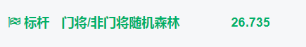
为什么会有两个结果？

　　这里解释一下，因为这里的标杆模型中的年龄的取值，是我以目前的时间为准，而不是以作者给的2018年为准，可能因为差了一岁导致球员的黄金年龄不同，价值也就不同。

随机森林调参（网格搜索）

#_*_coding:utf-8_*_
import pandas as pd
import numpy as np
import datetime as dt
from sklearn.ensemble import RandomForestRegressor

# 读取数据
train = pd.read_csv('data/train.csv')
test = pd.read_csv('data/test.csv')
submit = pd.read_csv('data/sample_submit.csv')

# 获得球员年龄
today = dt.datetime.today().year

train['birth_date'] = pd.to_datetime(train['birth_date'])
train['age'] = today - train.birth_date.dt.year

test['birth_date'] = pd.to_datetime(test['birth_date'])
test['age'] = today - test.birth_date.dt.year

# 获取球员最擅长位置的评分
positions = ['rw','rb','st','lw','cf','cam','cm','cdm','cb','lb','gk']

train['best_pos'] = train[positions].max(axis=1)
test['best_pos'] = test[positions].max(axis=1)

# 计算球员的身体质量指数（BMI）
train['BMI'] = 10000. * train['weight_kg'] / (train['height_cm'] ** 2)
test['BMI'] = 10000. * test['weight_kg'] / (test['height_cm'] ** 2)

# 判断一个球员是否是守门员
train['is_gk'] = train['gk'] > 0
test['is_gk'] = test['gk'] > 0

# 用多个变量准备训练随机森林
test['pred'] = 0
cols =  ['height_cm', 'weight_kg', 'potential', 'BMI', 'pac',
        'phy', 'international_reputation', 'age', 'best_pos']

# 用非守门员的数据训练随机森林
# 使用网格搜索微调模型
from sklearn.model_selection import GridSearchCV
param_grid = [
    {'n_estimators':[3,10,30], 'max_features':[2,4,6,8]},
    {'bootstrap':[False], 'n_estimators':[3,10],'max_features':[2,3,4]}
]
forest_reg = RandomForestRegressor()
grid_search = GridSearchCV(forest_reg, param_grid ,cv=5,
                           scoring='neg_mean_squared_error')

grid_search.fit(train[train['is_gk'] == False][cols] , train[train['is_gk'] == False]['y'])

preds = grid_search.predict(test[test['is_gk'] == False][cols])
test.loc[test['is_gk'] == False , 'pred'] = preds

# 用守门员的数据训练随机森林
# 使用网格搜索微调模型
from sklearn.model_selection import GridSearchCV
'''
先对estimators进行网格搜索，[3,10,30]
接着对最大深度max_depth 
内部节点再划分所需要最小样本数min_samples_split 进行网格搜索
最后对最大特征数,ax_features进行调参
'''
param_grid1 = [
    {'n_estimators':[3,10,30], 'max_features':[2,4,6,8]},
    {'bootstrap':[False], 'n_estimators':[3,10],'max_features':[2,3,4]}
]
'''
parm_grid 告诉Scikit-learn 首先评估所有的列在第一个dict中的n_estimators 和
max_features的 3*4=12 种组合，然后尝试第二个dict中的超参数2*3 = 6 种组合，
这次会将超参数bootstrap 设为False 而不是True（后者是该超参数的默认值）

总之，网格搜索会探索 12 + 6 = 18 种RandomForestRegressor的超参数组合，会训练
每个模型五次，因为使用的是五折交叉验证，换句话说，训练总共有18 *5 = 90 轮，、
将花费大量的时间，完成后，就可以得到参数的最佳组合了
'''
forest_reg1 = RandomForestRegressor()
grid_search1 = GridSearchCV(forest_reg, param_grid1 ,cv=5,
                           scoring='neg_mean_squared_error')

grid_search1.fit(train[train['is_gk'] == True][cols] , train[train['is_gk'] == True]['y'])

preds = grid_search1.predict(test[test['is_gk'] == True][cols])
test.loc[test['is_gk'] == True , 'pred'] = preds

# 输出预测值
submit['y'] = np.array(test['pred'])
submit.to_csv('my_RF_prediction1.csv',index = False)

# 打印参数的最佳组合
print(grid_search.best_params_)

　　

3，决策树标杆模型（四个特征）

整理此决策树训练模型的亮点

• 1，将出生年月日转化为球员的岁数（数据处理必须的）
• 2，将球员在各个位置的能力使用球员最擅长的位置表示（！！此处有待商榷）
• 3，直接使用潜力，国际知名度，年龄，最擅长位置评分这四个变量建立决策树（我觉得有点草率）

#_*_coding:utf-8_*_
import  pandas as pd
import datetime as dt
from sklearn.tree import DecisionTreeRegressor

# 读取数据
train = pd.read_csv('data/train.csv')
test = pd.read_csv('data/test.csv')
submit = pd.read_csv('data/sample_submit.csv')


# 获得球员年龄
today = dt.datetime.today().year

train['birth_date'] = pd.to_datetime(train['birth_date'])
train['age'] = today - train.birth_date.dt.year

test['birth_date'] = pd.to_datetime(test['birth_date'])
test['age'] = today - test.birth_date.dt.year

# 获得球员最擅长位置上的评分
positions = ['rw','rb','st','lw','cf','cam','cm','cdm','cb','lb','gk']

train['best_pos'] = train[positions].max(axis =1)
test['best_pos'] = test[positions].max(axis = 1)

# 用潜力，国际知名度，年龄，最擅长位置评分 这四个变量来建立决策树模型
col = ['potential','international_reputation','age','best_pos']

reg = DecisionTreeRegressor(random_state=100)
reg.fit(train[col],train['y'])

# 输出预测值
submit['y'] = reg.predict(test[col])
submit.to_csv('my_DT_prediction.csv',index=False)

　　结果如下：