Python_sklearn机器学习库学习笔记（五）k-means（聚类）

# K的选择：肘部法则

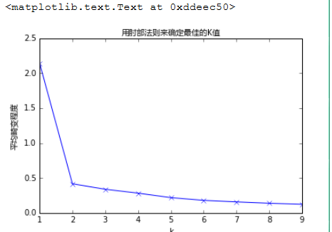
如果问题中没有指定 的值，可以通过肘部法则这一技术来估计聚类数量。肘部法则会把不同 值的
成本函数值画出来。随着 值的增大，平均畸变程度会减小；每个类包含的样本数会减少，于是样本
离其重心会更近。但是，随着 值继续增大，平均畸变程度的改善效果会不断减低。 值增大过程
中，畸变程度的改善效果下降幅度最大的位置对应的 值就是肘部。

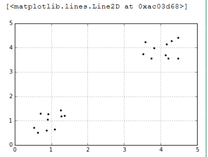
import numpy as np
import matplotlib.pyplot as plt
%matplotlib inline
#随机生成一个实数，范围在（0.5,1.5）之间
cluster1=np.random.uniform(0.5,1.5,(2,10))
cluster2=np.random.uniform(3.5,4.5,(2,10))
#hstack拼接操作
X=np.hstack((cluster1,cluster2)).T
plt.figure()
plt.axis([0,5,0,5])
plt.grid(True)
plt.plot(X[:,0],X[:,1],'k.')

 

%matplotlib inline
import matplotlib.pyplot as plt
from matplotlib.font_manager import FontProperties
font = FontProperties(fname=r"c:windowsfontsmsyh.ttc", size=10)

#coding:utf-8
#我们计算K值从1到10对应的平均畸变程度：
from sklearn.cluster import KMeans
#用scipy求解距离
from scipy.spatial.distance import cdist
K=range(1,10)
meandistortions=[]
for k in K:
    kmeans=KMeans(n_clusters=k)
    kmeans.fit(X)
    meandistortions.append(sum(np.min(
            cdist(X,kmeans.cluster_centers_,
                 'euclidean'),axis=1))/X.shape[0])
plt.plot(K,meandistortions,'bx-')
plt.xlabel('k')
plt.ylabel(u'平均畸变程度',fontproperties=font)
plt.title(u'用肘部法则来确定最佳的K值',fontproperties=font)

 

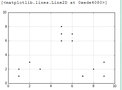
import numpy as np
x1 = np.array([1, 2, 3, 1, 5, 6, 5, 5, 6, 7, 8, 9, 7, 9])
x2 = np.array([1, 3, 2, 2, 8, 6, 7, 6, 7, 1, 2, 1, 1, 3])
X=np.array(list(zip(x1,x2))).reshape(len(x1),2)
plt.figure()
plt.axis([0,10,0,10])
plt.grid(True)
plt.plot(X[:,0],X[:,1],'k.')

from sklearn.cluster import KMeans
from scipy.spatial.distance import cdist
K=range(1,10)
meandistortions=[]
for k in K:
    kmeans=KMeans(n_clusters=k)
    kmeans.fit(X)
    meandistortions.append(sum(np.min(cdist(
            X,kmeans.cluster_centers_,"euclidean"),axis=1))/X.shape[0])
plt.plot(K,meandistortions,'bx-')
plt.xlabel('k')
plt.ylabel(u'平均畸变程度',fontproperties=font)
plt.title(u'用肘部法则来确定最佳的K值',fontproperties=font)

 

# 聚类效果的评价
#### 轮廓系数（Silhouette Coefficient）:s =ba/max(a, b)

import numpy as np
from sklearn.cluster import KMeans
from sklearn import metrics

plt.figure(figsize=(8,10))
plt.subplot(3,2,1)
x1 = np.array([1, 2, 3, 1, 5, 6, 5, 5, 6, 7, 8, 9, 7, 9])
x2 = np.array([1, 3, 2, 2, 8, 6, 7, 6, 7, 1, 2, 1, 1, 3])
X = np.array(list(zip(x1, x2))).reshape(len(x1), 2)
plt.xlim([0,10])
plt.ylim([0,10])
plt.title(u'样本',fontproperties=font)
plt.scatter(x1, x2)
colors = ['b', 'g', 'r', 'c', 'm', 'y', 'k', 'b']
markers = ['o', 's', 'D', 'v', '^', 'p', '*', '+']
tests=[2,3,4,5,8]
subplot_counter=1
for t in tests:
    subplot_counter+=1
    plt.subplot(3,2,subplot_counter)
    kmeans_model=KMeans(n_clusters=t).fit(X)
#     print kmeans_model.labels_:每个点对应的标签值
    for i,l in enumerate(kmeans_model.labels_):
        plt.plot(x1[i],x2[i],color=colors[l],
             marker=markers[l],ls='None')
        plt.xlim([0,10])
        plt.ylim([0,10])
        plt.title(u'K = %s, 轮廓系数 = %.03f' % 
                  (t, metrics.silhouette_score
                   (X, kmeans_model.labels_,metric='euclidean'))
                  ,fontproperties=font)

# 图像向量化

import numpy as np
from sklearn.cluster import KMeans
from sklearn.utils import shuffle
import mahotas as mh

original_img=np.array(mh.imread('tree.bmp'),dtype=np.float64)/255
original_dimensions=tuple(original_img.shape)
width,height,depth=tuple(original_img.shape)
image_flattend=np.reshape(original_img,(width*height,depth))

print image_flattend.shape
image_flattend

输出结果：

(102672L, 3L)

Out[96]:

array([[ 0.55686275,  0.57647059,  0.61960784],
       [ 0.68235294,  0.70196078,  0.74117647],
       [ 0.72156863,  0.7372549 ,  0.78039216],
       ..., 
       [ 0.75686275,  0.63529412,  0.46666667],
       [ 0.74117647,  0.61568627,  0.44705882],
       [ 0.70588235,  0.57647059,  0.40784314]])

 然后我们用K-Means算法在随机选择1000个颜色样本中建立64个类。每个类都可能是压缩调色板中的一种颜色

image_array_sample=shuffle(image_flattend,random_state=0)[:1000]
image_array_sample.shape
estimator=KMeans(n_clusters=64,random_state=0)
estimator.fit(image_array_sample)

#之后，我们为原始图片的每个像素进行类的分配
cluster_assignments=estimator.predict(image_flattend)

print cluster_assignments.shape
cluster_assignments

输出结果：

(102672L,)

Out[105]:

array([59, 39, 33, ..., 46,  8, 17])

#最后，我们建立通过压缩调色板和类分配结果创建压缩后的图片：
compressed_palette = estimator.cluster_centers_
compressed_img = np.zeros((width, height, compressed_palette.shape[1]))
label_idx = 0
for i in range(width):
    for j in range(height):
        compressed_img[i][j] = compressed_palette[cluster_assignments[label_idx]]
        label_idx += 1
plt.subplot(122)
plt.title('Original Image')
plt.imshow(original_img)
plt.axis('off')
plt.subplot(121)
plt.title('Compressed Image')
plt.imshow(compressed_img)
plt.axis('off')
plt.show()