7.2 径向基网络
7.2.1 RBF 网络
RBF网络是属于前馈神经网络,输入层与所有的其他神经网络相同,输入层到隐含层再到输出层经历了三次运算。
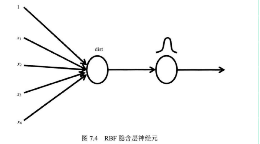
- 从输入层到隐含层求解输入节点与类别标签的欧式距离||dist||
- 在隐含层根据欧式距离使用RBF高斯函数进行曲线拟合
- 从隐含层到输出层为一个线性函数。如果是预测,则使用最小二乘法的正规方程组
与BP神经网络相比,RBF网络减少了误差反馈的权值更新环节,仅在隐含层使用高斯函数作为激活函数拟合数据的非线性,而网络调整是线性的,因而学习速率比BP网络要快的多,并能构避免局部极小问题。
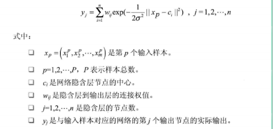
RBF径向基函数的激活函数如下:
RBF网络的架构如图:
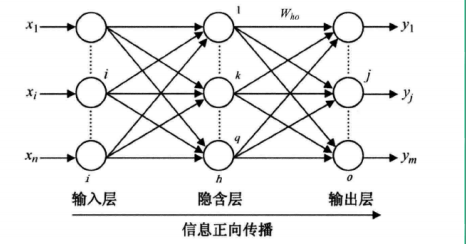
输入层、隐含层和输出层构成一个RBF神经网络。RBF网络结构与BP神经网络类似,也是一种三层网络。第一层是输入层,仅仅起到传输信号的作用,输入层和隐含层之间可以看作链接权值为1的链接。
第二层为隐含层,如用于预测,那么隐含层单元数与样本数应相同:从输入层到隐含层的变换是非线性的,通过激活函数(高斯函数)对样本进行调整。RBF的非线性函数包括两部分:首先对输入样本计算欧式距离;接下里对距离进行RBF拟合。
第三层为输出层,它一般是一个线性函数,对隐含层的输出数据进行线性权值调整,采用的线性优化模型。
7.2.2 代码实现:
(1)数据可视化,绘图函数。
# (1)绘制图形函数
def plotscatter(Xmat,Ymat,a,b,plt):
    fig = plt.figure()
    ax  = fig.add_subplot(111) #绘制图形位置
    ax.scatter(Xmat,Ymat,c='blue',marker='o')#绘制散点图
    plt.plot(Xmat,yhat,'r')
    plt.show()
(2)加载数据集
def loadDataSet(filename):     #加载数据集
    numFeat = len(open(filename).readline().split())-1
    X = [];Y = []
    fr = open(filename)
    for line in fr.readlines():
        curLine = line.strip().split(' ')
        X.append([float(curLine[i]) for i in xrange(numFeat)])
        Y.append(float(curLine[-1]))
    return X,Y
7.2.3 使用RBF预测
#局部加权线性回归算法
xArr,yArr = bmNet.loadDataSet("dataSet25.txt") #数据矩阵,分类标签

#RBF函数的平滑系数
miu = 0.02
k   = 0.03

#数据集坐标数组转换矩阵
xMat = mat(xArr);yMat = mat(yArr).T
testArr = xArr  #测试数组
m,n     = shape(xArr) #xArr的行数
yHat    = zeros(m)    #yHat是y的预测值,yHat的数据是y的回归线矩阵
for i in xrange(m):
    weights = mat(eye(m)) #权重矩阵
    for j in xrange(m):
        diffMat = testArr[i]-xMat[j,:]
        #利用RBF函数计算权重矩阵,计算后的权重是一个对角阵
        weights[j,j] = exp(diffMat*diffMat.T/(-miu*k**2))
    xTx = xMat.T*(weights*xMat)
    if linalg.det(xTx) != 0.0:    #行列式不为0
        ws = linalg.inv(Xmat.T*Xmat)*(Xmat.T*yHat)#矩阵的正规方程组的公式:inv(X.T*X)
        yHat[i] = testArr[i]*ws  #计算回归线坐标矩阵
    else:
        print "This matrix is sigular,cannot do inverse"
        sys.exit(0)#退出程序
plotscatter(xMat[:,1],yMat,yHat,plt)
完整代码:
from scipy import *
from scipy.linalg import norm, pinv

from matplotlib import pyplot as plt

class RBF:

    def __init__(self, indim, numCenters, outdim):
        self.indim = indim
        self.outdim = outdim
        self.numCenters = numCenters
        self.centers = [random.uniform(-1, 1, indim) for i in xrange(numCenters)]
        self.beta = 8
        self.W = random.random((self.numCenters, self.outdim))

    def _basisfunc(self, c, d):
        assert len(d) == self.indim
        return exp(-self.beta * norm(c-d)**2)

    def _calcAct(self, X):
        # calculate activations of RBFs
        G = zeros((X.shape[0], self.numCenters), float)
        for ci, c in enumerate(self.centers):
            for xi, x in enumerate(X):
                G[xi,ci] = self._basisfunc(c, x)
        return G

    def train(self, X, Y):
        """ X: matrix of dimensions n x indim
            y: column vector of dimension n x 1 """

        # choose random center vectors from training set
        rnd_idx = random.permutation(X.shape[0])[:self.numCenters]
        self.centers = [X[i,:] for i in rnd_idx]

        print "center", self.centers
        # calculate activations of RBFs
        G = self._calcAct(X)
        print G

        # calculate output weights (pseudoinverse)
        self.W = dot(pinv(G), Y)

    def test(self, X):
        """ X: matrix of dimensions n x indim """

        G = self._calcAct(X)
        Y = dot(G, self.W)
        return Y


if __name__ == '__main__':
    n = 100
    x = mgrid[-1:1:complex(0,n)].reshape(n, 1)
    # set y and add random noise
    y = sin(3*(x+0.5)**3 - 1)
    # y += random.normal(0, 0.1, y.shape)

    # rbf regression
    rbf = RBF(1, 10, 1)
    rbf.train(x, y)
    z = rbf.test(x)

    # plot original data
    plt.figure(figsize=(12, 8))
    plt.plot(x, y, 'k-')

    # plot learned model
    plt.plot(x, z, 'r-', linewidth=2)

    # plot rbfs
    plt.plot(rbf.centers, zeros(rbf.numCenters), 'gs')

    for c in rbf.centers:
        # RF prediction lines
        cx = arange(c-0.7, c+0.7, 0.01)
        cy = [rbf._basisfunc(array([cx_]), array([c])) for cx_ in cx]
        plt.plot(cx, cy, '-', color='gray', linewidth=0.2)

    plt.xlim(-1.2, 1.2)
    plt.show()
参考资料: 郑捷《机器学习算法原理与编程实践》 仅供学习研究