| 博客班级 | 机器学习 |
|---|---|
| 作业要求 | 作业链接 |
| 作业目标 | 感知器算法的理解及应用 |
| 学号 | 3180701214 |
一.实验目的
1.理解感知器算法原理,能实现感知器算法;
2.掌握机器学习算法的度量指标;
3.掌握最小二乘法进行参数估计基本原理;
4.针对特定应用场景及数据,能构建感知器模型并进行预测。
二.实验内容
1.安装Pycharm,注册学生版。
2.安装常见的机器学习库,如Scipy、Numpy、Pandas、Matplotlib,sklearn等。
3.编程实现感知器算法。
4.熟悉iris数据集,并能使用感知器算法对该数据集构建模型并应用
三.实验过程及结果
实验代码及注释
·Section 1
#导入pandas/numpy/matplotlib/sklearn机器学习库
import pandas as pd
import numpy as np
#导入iris数据集
from sklearn.datasets import load_iris
import matplotlib.pyplot as plt
%matplotlib inline  //使用%matplotlib命令可以将matplotlib的图表直接嵌入到Notebook之中,它的功能是可以内嵌绘图,并且可以省略掉plt.show()这一步
·Section 2
#load data
iris=load_iris()  //这里是sklearn中自带的一部分数据
df=pd.DataFrame(iris.data,columns=iris.feature_names)  //设置列名为iris.feature_names,iris.data(获取属性数据),iris.feature_names(获取列属性值)
df['label'] = iris.target  //增加一列为类别标签
·Section 3
#获取类别数据,这里注意的是已经经过处理,targe里0、1、2分别代表三种类别
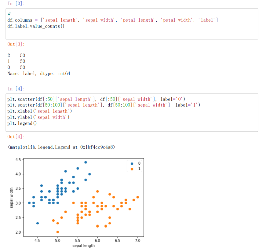
df.columns=['sepal length','sepal width','petal length','petal width','label'] //df的列标
df.label.value_counts(0) //计算series里面相同数据出现的频率(次数)
·Section 4
#画散点图,第一维数据作为x轴,第二维数据作为y轴,['sepal length','sepal width']特征分布查看
plt.scatter(df[:50]['sepal length'], df[:50]['sepal width'], label='0')  //绘制散点图
plt.scatter(df[50:100]['sepal length'], df[50:100]['sepal width'], label='1')
plt.xlabel('sepal length')  //给图加上图例
plt.ylabel('sepal width')
plt.legend()
·Section 5
data = np.array(df.iloc[:100, [0, 1, -1]]) //按行索引,提取前100行,取出第0,1,-1列
·Section 6
X, y = data[:,:-1], data[:,-1] //X为sepal length,sepal width y为标签
·Section 7
y = np.array([1 if i == 1 else -1 for i in y]) //将y的标签设置为1或者-1
·Section 8
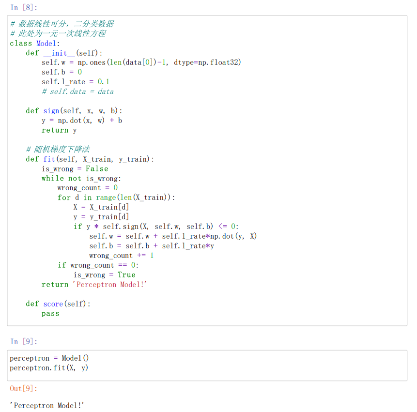
#数据线性可分,二分类数据
#此处为一元一次线性方程
class Model:
def init(self):  //将参数w1,w2置为1 b置为0 学习率为0.1
self.w = np.ones(len(data[0])-1, dtype=np.float32)  //data[0]为第一行的数据len(data[0]=3)这里取两个w权重参数
self.b = 0
self.l_rate = 0.1
%# self.data = data

def sign(self, x, w, b):
y = np.dot(x, w) + b
return y

#随机梯度下降法
def fit(self, X_train, y_train):  //拟合训练数据求w和b
is_wrong = False  //判断是否误分类
while not is_wrong:
wrong_count = 0
for d in range(len(X_train)):  //取出样例,不断的迭代
X = X_train[d]
y = y_train[d]
if y * self.sign(X, self.w, self.b) <= 0:  //根据错误的样本点不断的更新和迭代w和b的值(根据相乘结果是否为负来判断是否出错,本题将0也归为错误)
self.w = self.w + self.l_ratenp.dot(y, X)
self.b = self.b + self.l_ratey
wrong_count += 1
if wrong_count == 0:  //直到误分类点为0 跳出循环
is_wrong = True
return 'Perceptron Model!'

def score(self):
pass
·Section 9
perceptron = Model()
perceptron.fit(X, y)  //感知机模型
·Section 10
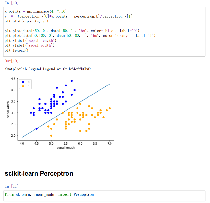
#绘制模型图像,定义一些基本的信息
x_points = np.linspace(4, 7,10)  //x轴的划分
y_ = -(perceptron.w[0]*x_points + perceptron.b)/perceptron.w[1]
plt.plot(x_points, y_)  //绘制模型图像(数据、颜色、图例等信息)
plt.plot(data[:50, 0], data[:50, 1], 'bo', color='blue', label='0')
plt.plot(data[50:100, 0], data[50:100, 1], 'bo', color='orange', label='1')
plt.xlabel('sepal length')
plt.ylabel('sepal width')
plt.legend()
·Section 11
from sklearn.linear_model import Perceptron //定义感知机(下面将使用感知机)
·Section 12
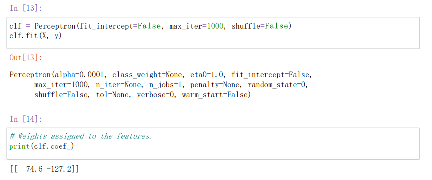
"""自定义感知机"""
clf = Perceptron(fit_intercept=False, max_iter=1000, shuffle=False)
"""使用训练数据进行训练"""
clf.fit(X, y)
·Section 13
%# Weights assigned to the features.
print(clf.coef_)  //输出感知机模型参数
·Section 14
%# 截距 Constants in decision function.
print(clf.intercept_)//输出感知机模型参数
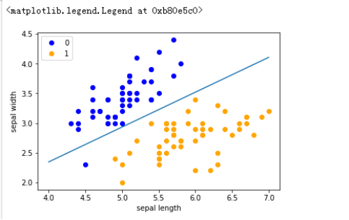
·Section 15
x_ponits = np.arange(4, 8)  //确定x轴和y轴的值
y_ = -(clf.coef_[0][0]*x_ponits + clf.intercept_)/clf.coef_[0][1]
plt.plot(x_ponits, y_)  //确定拟合的图像的具体信息(数据点,线,大小,粗细颜色等内容)
plt.plot(data[:50, 0], data[:50, 1], 'bo', color='blue', label='0')
plt.plot(data[50:100, 0], data[50:100, 1], 'bo', color='orange', label='1')
plt.xlabel('sepal length')
plt.ylabel('sepal width')
plt.legend()
实验结果截图
四.作业小结
1.psp表格
| psp2.1 | 任务内容 | 计划完成需要的时间(min) | 实际完成需要的时间(min) |
|---|---|---|---|
| Planning | 计划 | 120 | 8 |
| Development | 开发 | 100 | 150 |
| Analysis | 需求分析(包括学习新技术) | 10 | 10 |
| Design Spec | 生成设计文档 | 30 | 40 |
| Design Review | 设计复审 | 5 | 10 |
| Coding Standard | 代码规范 | 3 | 2 |
| Design | 具体设计 | 10 | 12 |
| Coding | 具体编码 | 36 | 21 |
| Code Review | 代码复审 | 5 | 7 |
| Test | 测试(自我测试,修改代码,提交修改) | 10 | 15 |
| Reporting | 报告 | 9 | 6 |
| Test Report | 测试报告 | 3 | 2 |
| Size Measurement | 计算工作量 | 2 | 1 |
| Postmortem & Process Improvement Plan | 事后总结,并提出过程改进计划 | 3 | 3 |
2.心得和经验
通过本次实验,我理解了感知器算法原理,知道了感知器收敛的前提是两个类别必须是线性可分的,且学习率足够小。如果两个类别无法通过一个线性决策边界进行划分,我们可以设置一个迭代次数或者一个判断错误样本的阈值,否则感知器算法会一直运行下去。对于x和y的n对观察值,用于描述其关系的直线有多条,究竟用哪条直线来代表两个变量之间的关系,需要有一个明确的原则。这时用距离各观测点最近的一条直线,用它来代表x与y之间的关系与实际数据的误差比其它任何直线都小,而根据这一思想求得直线中未知常数的方法就是最小二乘法,即因变量的观察值与估计值之间的离差平方和达到最小来求得和的方法。同时还熟悉了iris数据集,能使用感知器算法对该数据集构建模型并应用。