几何和线性代数算子
Geometry and Linear Algebraic Operations
了解了线性代数的基础知识,并了解了如何使用来表示转换数据的常见操作。线性代数是进行深度学习和更广泛的机器学习的主要数学支柱之一。虽然包含了足够多的机制来交流现代深度学习模型的机制,但是这个主题还有很多内容。将更深入地介绍线性代数运算的一些几何解释,并介绍一些基本概念,包括特征值和特征向量。
1. Geometry of Vectors
首先,需要讨论向量的两种常见的几何解释,即空间中的点或方向。基本上,向量是一个数字列表,如下面的Python列表。
v = [1, 7, 0, 1]
数学家通常把写成列向量或行向量,也就是说
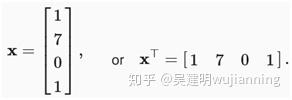
通常有不同的解释,其中数据点是列向量,用于形成加权和的权重是行向量。然而,保持灵活性是有益的。矩阵是有用的数据结构:允许组织具有不同变化模式的数据。例如,矩阵中的行可能对应于不同的房屋(数据点),而列可能对应于不同的属性。如果曾经使用过电子表格软件或阅读过这些内容,这听起来应该很熟悉。因此,虽然单个向量的默认方向是列向量,但在表示表格数据集的矩阵中,将每个数据点视为矩阵中的行向量更为传统。而且,正如将在后面几章中看到的,这项公约将使共同的深入学习实践成为可能。例如,沿着张量的最外轴,可以访问或枚举数据点的小批量,如果没有小批量,则只访问或枚举数据点。
给定一个向量,首先要解释的是空间中的一个点。在二维或三维空间中,可以通过使用向量的分量来定义这些点在空间中的位置,与称为原点的固定参考相比。如图1所示。
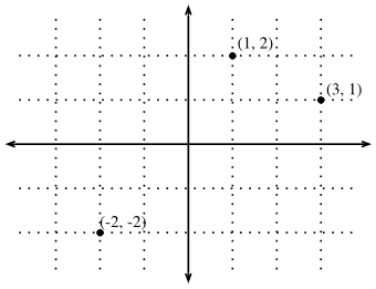
Fig. 1. An illustration of visualizing vectors as points in the plane. The first component of the vector gives the x-coordinate, the second component gives the y-coordinate. Higher dimensions are analogous, although much harder to visualize.
这种几何观点使能够在更抽象的层面上考虑这个问题。不再面临一些难以逾越的表面问题,如将图片分类为猫或狗,可以开始抽象地将任务视为空间中点的集合,并将任务想象为发现如何分离两个不同的点簇。
同时,还有第二种观点,人通常把矢量当作空间的方向。不仅能想到矢量v=[2,3]⊤ 作为位置2右边的单位和3单位从原点向上,也可以把看作是自己要走的方向2往右边走3站起来。这样,认为图2中的所有向量都是相同的。
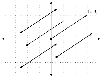
Fig. 2. Any vector can be visualized as an arrow in the plane. In this case, every vector drawn is a representation of the vector (2,3).
这种转变的好处之一是可以从视觉上理解向量加法的行为。特别是,遵循一个向量给出的方向,然后遵循另一个向量给出的方向,如图3所示。
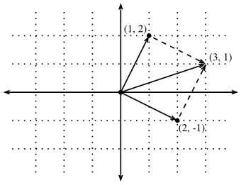
Fig. 3. We can visualize vector addition by first following one vector, and then another.
向量减法也有类似的解释。考虑到u=v+(u−v)u=v+(u−v),,看到矢量u−v是从这一点出发的方向u到点v。
2. Dot Products and Angles
如果取两个列向量u和v,可以通过计算形成点积:
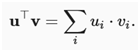
因为上式是对称的,将镜像乘法运算:
为了强调这样一个事实,交换向量的顺序将得到相同的答案。
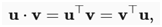
点积也允许几何解释:与两个向量之间的角度密切相关。考虑图4所示的角度。
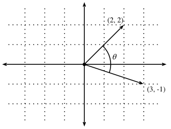
Fig. 4. Between any two vectors in the plane there is a well defined angle θθ. We will see this angle is intimately tied to the dot product.
首先,让考虑两个特定的向量:
v=(r,0) and w=(scos(θ), ssin(θ)).
矢量v是长度,并与x轴和向量w,长度为s,以一定角度θ和x轴,如果计算这两个向量的点积,会看到
v⋅w=rscos(θ)=∥v∥∥w∥cos(θ).
通过一些简单的代数操作,可以重新排列项以获得
简言之,对于这两个特定的向量,点积和范数的结合告诉两个向量之间的角度。一般来说,这同样的事实是正确的。但是,如果考虑写作的话,不会在这里推导出这个表达式

,有两种方法:一种是用点积,另一种是几何上用余弦定律,可以得到完整的关系。实际上,对于任何两个向量v和w,两个矢量之间的夹角为
这是一个很好的结果,因为计算中没有提到二维。事实上,可以毫无疑问地在三百万或三百万个维度上使用。
作为一个简单的例子,让看看如何计算一对向量之间的角度:
%matplotlib inline
from d2l import mxnet as d2l
from IPython import display
from mxnet import gluon, np, npx
npx.set_np()
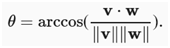
def angle(v, w):
return np.arccos(v.dot(w) / (np.linalg.norm(v) * np.linalg.norm(w)))
angle(np.array([0, 1, 2]), np.array([2, 3, 4]))
array(0.41899002)
We will not use it right now, but it is useful to know that we will refer to vectors for which the angle is π/2π/2 (or equivalently 90∘90∘) as being orthogonal. By examining the equation above, we see that this happens when θ=π/2θ=π/2, which is the same thing as cos(θ)=0cos(θ)=0. The only way this can happen is if the dot product itself is zero, and two vectors are orthogonal if and only if v⋅w=0v⋅w=0. This will prove to be a helpful formula when understanding objects geometrically.
It is reasonable to ask: why is computing the angle useful? The answer comes in the kind of invariance we expect data to have. Consider an image, and a duplicate image, where every pixel value is the same but 10%10% the brightness. The values of the individual pixels are in general far from the original values. Thus, if one computed the distance between the original image and the darker one, the distance can be large.
However, for most ML applications, the content is the same—it is still an image of a cat as far as a cat/dog classifier is concerned. However, if we consider the angle, it is not hard to see that for any vector vv, the angle between vv and 0.1⋅v0.1⋅v is zero. This corresponds to the fact that scaling vectors keeps the same direction and just changes the length. The angle considers the darker image identical.
Examples like this are everywhere. In text, we might want the topic being discussed to not change if we write twice as long of document that says the same thing. For some encoding (such as counting the number of occurrences of words in some vocabulary), this corresponds to a doubling of the vector encoding the document, so again we can use the angle.
2.1. Cosine Similarity
In ML contexts where the angle is employed to measure the closeness of two vectors, practitioners adopt the term cosine similarity to refer to the portion
The cosine takes a maximum value of 11 when the two vectors point in the same direction, a minimum value of −1−1 when they point in opposite directions, and a value of 00 when the two vectors are orthogonal. Note that if the components of high-dimensional vectors are sampled randomly with mean 00, their cosine will nearly always be close to 00.
3. Hyperplanes
In addition to working with vectors, another key object that you must understand to go far in linear algebra is the hyperplane, a generalization to higher dimensions of a line (two dimensions) or of a plane (three dimensions). In an dd-dimensional vector space, a hyperplane has d−1d−1 dimensions and divides the space into two half-spaces.
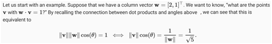
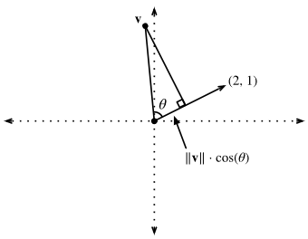
Fig. 5. Recalling trigonometry, we see the formula ∥v∥cos(θ)‖v‖cos(θ) is the length of the projection of the vector vv onto the direction of ww
If we consider the geometric meaning of this expression, we see that this is equivalent to saying that the length of the projection of vv onto the direction of ww is exactly 1/∥w∥1/‖w‖, as is shown in :numref:fig_vector-project. The set of all points where this is true is a line at right angles to the vector ww. If we wanted, we could find the equation for this line and see that it is 2x+y=12x+y=1 or equivalently y=1−2xy=1−2x.
If we now look at what happens when we ask about the set of points with w⋅v>1w⋅v>1 or w⋅v<1w⋅v<1, we can see that these are cases where the projections are longer or shorter than 1/∥w∥1/‖w‖, respectively. Thus, those two inequalities define either side of the line. In this way, we have found a way to cut our space into two halves, where all the points on one side have dot product below a threshold, and the other side above as we see in Fig.6.
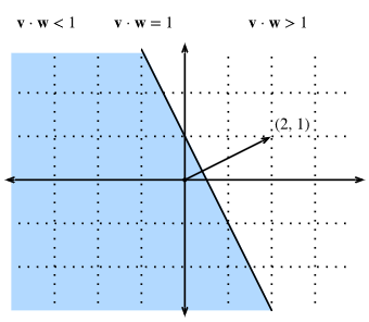
Fig. 6. If we now consider the inequality version of the expression, we see that our hyperplane (in this case: just a line) separates the space into two halves.
The story in higher dimension is much the same. If we now take w=[1,2,3]⊤w=[1,2,3]⊤ and ask about the points in three dimensions with w⋅v=1w⋅v=1, we obtain a plane at right angles to the given vector ww. The two inequalities again define the two sides of the plane as is shown in Fig..7.

Fig. 7 Hyperplanes in any dimension separate the space into two halves.
While our ability to visualize runs out at this point, nothing stops us from doing this in tens, hundreds, or billions of dimensions. This occurs often when thinking about machine learned models. For instance, we can understand linear classification models, as methods to find hyperplanes that separate the different target classes. In this context, such hyperplanes are often referred to as decision planes. The majority of deep learned classification models end with a linear layer fed into a softmax, so one can interpret the role of the deep neural network to be to find a non-linear embedding such that the target classes can be separated cleanly by hyperplanes.
To give a hand-built example, notice that we can produce a reasonable model to classify tiny images of t-shirts and trousers from the Fashion MNIST dataset by just taking the vector between their means to define the decision plane and eyeball a crude threshold. First we will load the data and compute the averages.
# Load in the dataset
train = gluon.data.vision.FashionMNIST(train=True)
test = gluon.data.vision.FashionMNIST(train=False)
X_train_0 = np.stack([x[0] for x in train if x[1] == 0]).astype(float)
X_train_1 = np.stack([x[0] for x in train if x[1] == 1]).astype(float)
X_test = np.stack(
[x[0] for x in test if x[1] == 0 or x[1] == 1]).astype(float)
y_test = np.stack(
[x[1] for x in test if x[1] == 0 or x[1] == 1]).astype(float)
# Compute averages
ave_0 = np.mean(X_train_0, axis=0)
ave_1 = np.mean(X_train_1, axis=0)
It can be informative to examine these averages in detail, so let us plot what they look like. In this case, we see that the average indeed resembles a blurry image of a t-shirt.
# Plot average t-shirt
d2l.set_figsize()
d2l.plt.imshow(ave_0.reshape(28, 28).tolist(), cmap='Greys')
d2l.plt.show()

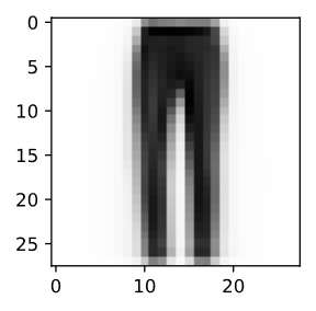
In the second case, we again see that the average resembles a blurry image of trousers.
# Plot average trousers
d2l.plt.imshow(ave_1.reshape(28, 28).tolist(), cmap='Greys')
d2l.plt.show()
In a fully machine learned solution, we would learn the threshold from the dataset. In this case, I simply eyeballed a threshold that looked good on the training data by hand.
# Print test set accuracy with eyeballed threshold
w = (ave_1 - ave_0).T
predictions = X_test.reshape(2000, -1).dot(w.flatten()) > -1500000
# Accuracy
np.mean(predictions.astype(y_test.dtype) == y_test, dtype=np.float64)
array(0.801, dtype=float64)