数据分析核心包 - pandas
pandas简介
pandas是一个强大的Python数据分析的工具包,是基于NumPy构建的。
pandas的主要功能
具备对其功能的数据结构DataFrame,Series
集成时间序列功能
提供丰富的数学运作和操作
灵活处理缺失数据
安装方法:pip install pandas
引用方法:import pandas as pd
1,Series
1,Series - 一维数据对象
Series是一种类似于一位数组的对象,由一组数据和一组与之相关的数据标签(索引)组成。
创建方式:
sr0 = pd.Series([4, 7, -5, 3])
sr1 = pd.Series([4, 7, -5, 3], index = ['a', 'b', 'c', 'd'])  # 自设索引,依然可以通过数字索引进行访问
sr3 = pd.Series({'a': 1, 'b':2})
sr4 = pd.Series(0, index = ['a', 'b', 'c', 'd'])  # 通过字典创建标签
获取值数组和索引数组:values属性和index属性
Series表较像列表(数组)和字典的结合体
2,Series - 使用特性
| Series支持array的特性(下标) | Series支持字典的特性(标签) | ||
| 从ndarry创建Series | Series(arr) | 从字典创建Series | Series(dic) |
| 与标量运算 | sr*2 | in运算 | 'a' in sr |
| 两个Series运算 | sr1+sr2 | 键索引 | sr['a'], sr[['a', 'b', 'd']] |
| 索引 | sr[0], sr[[1,2,4]] | ||
| 切片 | sr[0:2] | ||
| 通用函数 | np.abs(sr) | ||
| 布尔值过滤 | sr[sr>0] | ||
示例:
In [13]: sr = pd.Series([2,3,4,5],index = ['a','b','c','d'])   # 可以另设置索引。

In [14]: sr.index
Out[14]: Index(['a', 'b', 'c', 'd'], dtype='object')  # 打印索引

In [15]: for i in sr:
    ...:     print(i)
    ...:
3,Series - 整数索引
例如:
sr = pd.Series(np.arange(4.))
sr[-1]
如果索引使整数类型,则根据整数进行下标获取值时总是面向标签的。
解决方法:loc属性(将索引解释为标签)和iloc属性(将索引解释为下标)
4,Series - 数据对齐
##例
sr1 = pd.Series([12, 23, 34],index = ['c', 'a', 'd'])
sr2 = pd.Series([11, 20, 10],index = ['d', 'c', 'a'])
sr1 + sr2
①pandas在进行两个Series对象的运算时,会按索引进行对齐然后计算。
②如果两个Series对象的索引不完全相同,则结果的索引是两个操作数索引的并集。
如果只有一个对象在某索引下有值,则结果中该索引的值为nan(缺失值)
③如何使结果在索引'b'处的值为11,在索引'd'处的值为34?
灵活的算术方法:add, sub, div, mul
sr1.add(sr2,fill_value = 0)
5,Series - 缺失数据
①缺失数据:使用NaN(Not a Number)来表示缺失数据。其值等于np.nan。内置的None值也会被当作NaN处理。
②处理缺失数据的相关方法:
dropna()  # 过滤掉值为NaN的行
fillna()     # 填充缺失的数据
isnull()     # 返回布尔数组,缺失值对应为True
notnull()  # 返回布尔数组,缺失值对应为False
③过滤缺失数据:sr.dropna() 或 sr[data.natnull()]
④填充缺失数据:fillna(0)
2,DataFrame
1,DataFrame-二维数据对象
DataFrame是一个表格型的数据结构,含有一组有序的列。DataFrame可以被看做是由Series组成的字典,并且共用一个索引。
创建方式:
pd.DataFrame({'one':[1, 2, 3, 4],'two':[4, 3, 2, 1]})
pd.DataFrame({'one':pd.Series([1, 2, 3], index = ['a', 'b', 'c']),
'two':pd.Series([1, 2, 3, 4], index = ['b', 'a', 'c', 'd'])})
...
csv文件读取与写入:
df.read_csv('filename.csv')
df.to_csv()
2,DataFrame - 常用属性
| DataFrame常用属性 | |
| index | 获取索引 |
| T | 转置 |
| columns | 获取列索引 |
| values | 获取值数组 |
| describe() | 获取快速统计 |
3,DataFrame - 索引和切片
DataFrame是一个二维数据类型,所以有行索引和列索引
DataFrame同样可以通过标签和位置两种方法进行索引和切片
loc(标签)属性和iloc(下标)属性:
使用方法:逗号隔开,前面是行索引,后面是列索引
行/列索引部分可以是常规索引,切片,布尔值索引,花式索引任意搭配
In [89]: df
Out[89]:
   one  two
a  1.0    2
b  2.0    1
c  3.0    3
d  NaN    4

In [90]: df['one']['a']   # 此处先选列,后选行。
Out[90]: 1.0

# 标签或者下标选取

# 标签选取
In [91]: df.loc['a','one']  # 先行后列,推荐使用该方式。
Out[91]: 1.0

# 可以单独查看列,不能单独查看行
# 实现方式:该格式相当于每一列为一个series,然后多个series拼接在一起,故此。
In [93]: df['one']
Out[93]:
a    1.0
b    2.0
c    3.0
d    NaN
Name: one, dtype: float64

# 单独查看行方式:
In [96]: df.loc['a',:]  # 行通过a,列通过分号选择所有的列。
Out[96]:
one    1.0
two    2.0
Name: a, dtype: float64

In [97]: df.loc[['a','c'],:]
Out[97]:
one two
a 1.0 2
c 3.0 3
4,DataFrame数据对齐与缺失数据
DataFrame对象在运算时,同样会进行数据对齐,其行索引和列索引分别对齐。
DataFrame处理缺失数据的相关方法:
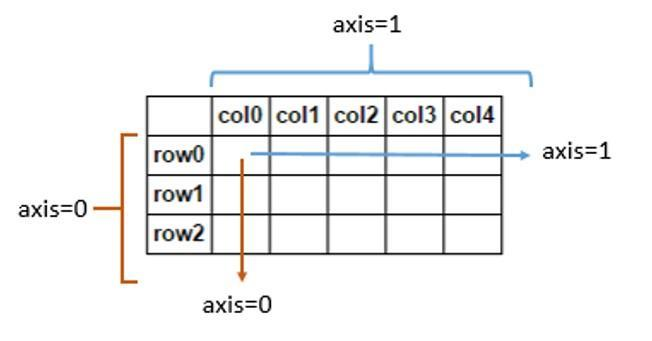
dropna(axis = 0,where = 'any',...)  # axis=0代表往跨行(down),而axis=1代表跨列(across)
fillna()
isnull()
notnull()
①详解axis
axis=0代表往跨行(down),而axis=1代表跨列(across)
轴用来为超过一维的数组定义的属性,二维数据拥有两个轴:第0轴沿着行的方向垂直往下,第1轴沿着列的方向水平延伸
In [125]: df
Out[125]:
two one
c NaN 4
d 2.0 5
b 3.0 6
a 4.0 7

In [126]: df.dropna(axis = 1)  # 删除存在nan值的列。axis = 1时表示纵轴,也即列。
Out[126]:
one
c 4
d 5
b 6
a 7

In [127]: df.dropna(axis = 0)  # 删除存在nan值的行。axis = 0时表示横轴,也即行。
Out[127]:
two one
d 2.0 5
b 3.0 6
a 4.0 7
②数据对齐:
In [97]: df
Out[97]:
   one  two
a  1.0    2
b  2.0    1
c  3.0    3
d  NaN    4

In [98]: df = pd.DataFrame({'two':[1,2,3,4],'one':[4,5,6,7]},index = ['c','d','b','a'])

In [99]: df2 = _95

In [100]: df
Out[100]:
   two  one
c    1    4
d    2    5
b    3    6
a    4    7

In [101]: df2
Out[101]:
   one  two
a  1.0    2
b  2.0    1
c  3.0    3
d  NaN    4

In [102]: df + df2
Out[102]:
   one  two
a  8.0    6
b  8.0    4
c  7.0    4
d  NaN    6
③处理数据缺失相关方法示例:
In [103]: df2
Out[103]:
   one  two
a  1.0    2
b  2.0    1
c  3.0    3
d  NaN    4

In [104]: df2.fillna(0)
Out[104]:
   one  two
a  1.0    2
b  2.0    1
c  3.0    3
d  0.0    4

In [105]: df2.dropna()  # 默认处理方法,若有缺失值,则删掉该行。
Out[105]:
   one  two
a  1.0    2
b  2.0    1
c  3.0    3

In [106]: df2.isnull()
Out[106]:
     one    two
a  False  False
b  False  False
c  False  False
d   True  False

In [107]: df2.notnull()
Out[107]:
     one   two
a   True  True
b   True  True
c   True  True
d  False  True
④dropna其他情况用法:
In [117]: df2
Out[117]:
   one  two
a  1.0  2.0
b  2.0  1.0
c  3.0  3.0
d  NaN  4.0

In [118]: df2.loc['c',:] = np.nan

In [119]: df2
Out[119]:
   one  two
a  1.0  2.0
b  2.0  1.0
c  NaN  NaN
d  NaN  4.0

In [120]: df2.dropna(how = 'all')  # 删除数据全是nan的行
Out[120]:
   one  two
a  1.0  2.0
b  2.0  1.0
d  NaN  4.0

In [121]: df2.dropna(how = 'any')  # 删除数据有nan的行
Out[121]:
   one  two
a  1.0  2.0
b  2.0  1.0

In [125]: df
Out[125]:
two one
c NaN 4
d 2.0 5
b 3.0 6
a 4.0 7

In [126]: df.dropna(axis = 1)  # 删除存在nan值的列。axis = 1时表示纵轴,也即列。
Out[126]:
one
c 4
d 5
b 6
a 7

In [127]: df.dropna(axis = 0)  # 删除存在nan值的行。axis = 0时表示横轴,也即行。
Out[127]:
two one
d 2.0 5
b 3.0 6
a 4.0 7
3,pandas其他常用对象
1,pandas - 其他常用方法
NumPy的通用函数同样适用于pandas
| pandas - 其他常用方法 | |
| mean(axis = 0,skipna = False) | 对列(行)求平均值 |
| sum(axis = 1) | 对列(行)求和 |
| sort_index(axis, ..., ascending) | 对列(行)索引排序 |
| sort_values(by, axis, ascending) | 按某一列(行)的值排序 |
| apply(func, axis = 0) |
将自定义函数应用在各行或者列上, func可返回标量或者Series |
| applymap(func) | 将函数应用在DataFrame各个元素上 |
| map(func) | 将函数应用在Series各个元素上 |
①求平均值求和代码示例
In [125]: df
Out[125]:
   two  one
c  NaN    4
d  2.0    5
b  3.0    6
a  4.0    7

# 求平均值
# 因为DataFrame对象有两列,所以mean方法返回的是长度为2的series对象。
In [129]: df.mean()  # 默认以行显示求每一列的平均值
Out[129]:
two    3.0
one    5.5
dtype: float64

In [130]: df.mean(axis = 1)  # 当加入参数axis = 1时,表示跨列计算显示每一行的平均值
Out[130]:
c    4.0
d    3.5
b    4.5
a    5.5
dtype: float64

# 求和
In [131]: df.sum()  # 默认求每一列的平均值
Out[131]:
two     9.0
one    22.0
dtype: float64

In [133]: df.sum(axis = 1)  # 跨列计算显示每一行的和。
Out[133]:
c     4.0
d     7.0
b     9.0
a    11.0
dtype: float64
②排序
In [134]: df
Out[134]:
   two  one
c  NaN    4
d  2.0    5
b  3.0    6
a  4.0    7

# 排序

In [135]: df.sort_values(by = 'two')  # 按照某一列来排序,降序。
Out[135]:
   two  one
d  2.0    5
b  3.0    6
a  4.0    7
c  NaN    4

In [139]: df.sort_values(by = 'two',ascending=False)  #倒序,升序。(将参数False改成True,则为降序)
Out[139]:
   two  one
a  4.0    7
b  3.0    6
d  2.0    5
c  NaN    4

In [141]: df.sort_values(by = 'a',ascending=False,axis = 1) #以行排序(跨列以a行进行排序)
Out[141]:
   one  two
c    4  NaN
d    5  2.0
b    6  3.0
a    7  4.0

In [143]: df.sort_values(by = 'two',ascending=False,axis = 0)  # 以列排序
Out[143]:
   two  one
a  4.0    7
b  3.0    6
d  2.0    5
c  NaN    4

# 索引排序
In [145]: df.sort_index()  # 按照标签索引来排序,默认升序
Out[145]:
two one
a 4.0 7
b 3.0 6
c NaN 4
d 2.0 5

In [146]: df.sort_index(ascending = False)  # 按照降序进行索引排序
Out[146]:
   two  one
d  2.0    5
c  NaN    4
b  3.0    6
a  4.0    7

In [147]: df.sort_index(ascending = False ,axis =1)  # 跨列进行行排序,t在o之前。
Out[147]:
   two  one
c  NaN    4
d  2.0    5
b  3.0    6
a  4.0    7
备注:
若排序中出现了NaN,则将此行放置最后,不参与排序。
2,pandas - 时间对象处理
①时间序列类型:
时间戳:特定时刻
固定时期:如2018年12月
时间间隔:起始时间-结束时间
| Python标准库处理时间对象 | datatime |
| 灵活处理时间对象 | ①datautil |
| ②datautil.parser.parse() | |
| 成组处理时间对象 | ①pandas |
| ②pd.to_datatime() |
②产生时间对象数组:
| 产生时间对象数组:date_range | |
| start | 开始时间 |
| end | 结束时间 |
| periods | 时间长度 |
| freq |
时间频率 默认为'D',可选H(our),W(eek),B(usiness),S(emi-)M(onth), M(min)T(es),S(econd),A(year),... |
代码示例:
In [149]: import datetime  # 导入python标准库处理时间对象:datetime

In [150]: import dateutil  # 导入灵活处理时间对象:dateutil

In [151]: datetime.datetime.strptime('2010-01-01','%Y-%m-%d')  # 标准库,需要符合书写规范
Out[151]: datetime.datetime(2010, 1, 1, 0, 0)

# 灵活处理时间对象:可以改变自身输入格式,也可得到结果
In [152]: dateutil.parser.parse('2001/02/03')
Out[152]: datetime.datetime(2001, 2, 3, 0, 0)

In [153]: dateutil.parser.parse('2001-02-03')
Out[153]: datetime.datetime(2001, 2, 3, 0, 0)

In [154]: dateutil.parser.parse('2001-FEB-03')
Out[154]: datetime.datetime(2001, 2, 3, 0, 0)

In [155]: dateutil.parser.parse('02/03/2001')
Out[155]: datetime.datetime(2001, 2, 3, 0, 0)

# to_datetime 批量的字符串列表转换成datetime对象的数组或者索引
In [3]: pd.to_datetime(['2018-12-12','2018/11/11'])
Out[3]: DatetimeIndex(['2018-12-12', '2018-11-11'], dtype='datetime64[ns]', freq=None)

# date_range

In [6]: pd.date_range(start = '2018/11/11',end = '2018/12/12')
Out[6]:
DatetimeIndex(['2018-11-11', '2018-11-12', '2018-11-13', '2018-11-14',
               '2018-11-15', '2018-11-16', '2018-11-17', '2018-11-18',
               '2018-11-19', '2018-11-20', '2018-11-21', '2018-11-22',
               '2018-11-23', '2018-11-24', '2018-11-25', '2018-11-26',
               '2018-11-27', '2018-11-28', '2018-11-29', '2018-11-30',
               '2018-12-01', '2018-12-02', '2018-12-03', '2018-12-04',
               '2018-12-05', '2018-12-06', '2018-12-07', '2018-12-08',
               '2018-12-09', '2018-12-10', '2018-12-11', '2018-12-12'],
              dtype='datetime64[ns]', freq='D')

In [7]: pd.date_range('2018/11/11','2018/12/12')  # 可以省略start和end
Out[7]:
DatetimeIndex(['2018-11-11', '2018-11-12', '2018-11-13', '2018-11-14',
               '2018-11-15', '2018-11-16', '2018-11-17', '2018-11-18',
               '2018-11-19', '2018-11-20', '2018-11-21', '2018-11-22',
               '2018-11-23', '2018-11-24', '2018-11-25', '2018-11-26',
               '2018-11-27', '2018-11-28', '2018-11-29', '2018-11-30',
               '2018-12-01', '2018-12-02', '2018-12-03', '2018-12-04',
               '2018-12-05', '2018-12-06', '2018-12-07', '2018-12-08',
               '2018-12-09', '2018-12-10', '2018-12-11', '2018-12-12'],
              dtype='datetime64[ns]', freq='D')

In [8]: pd.date_range(start = '2018/11/11',periods = 8)  # 起始,时间间隔是八天
Out[8]:
DatetimeIndex(['2018-11-11', '2018-11-12', '2018-11-13', '2018-11-14',
               '2018-11-15', '2018-11-16', '2018-11-17', '2018-11-18'],
              dtype='datetime64[ns]', freq='D')

In [9]: pd.date_range(end = '2018/11/11',periods = 8)  # 结束,时间间隔是八天
Out[9]:
DatetimeIndex(['2018-11-04', '2018-11-05', '2018-11-06', '2018-11-07',
               '2018-11-08', '2018-11-09', '2018-11-10', '2018-11-11'],
              dtype='datetime64[ns]', freq='D')

In [10]: pd.date_range('2018/11/11',periods = 8,freq = 'B')  # 工作日
Out[10]:
DatetimeIndex(['2018-11-12', '2018-11-13', '2018-11-14', '2018-11-15',
               '2018-11-16', '2018-11-19', '2018-11-20', '2018-11-21'],
              dtype='datetime64[ns]', freq='B')

In [11]: pd.date_range('2018/11/11',periods = 8,freq = 'H')  # 时间间隔为小时,也可以是1h20min等
Out[11]:
DatetimeIndex(['2018-11-11 00:00:00', '2018-11-11 01:00:00',
               '2018-11-11 02:00:00', '2018-11-11 03:00:00',
               '2018-11-11 04:00:00', '2018-11-11 05:00:00',
               '2018-11-11 06:00:00', '2018-11-11 07:00:00'],
              dtype='datetime64[ns]', freq='H')

In [12]: pd.date_range('2018/11/11',periods = 8,freq = 'W')  # W:星期,默认周日开始
Out[12]:
DatetimeIndex(['2018-11-11', '2018-11-18', '2018-11-25', '2018-12-02',
               '2018-12-09', '2018-12-16', '2018-12-23', '2018-12-30'],
              dtype='datetime64[ns]', freq='W-SUN')

In [13]: pd.date_range('2018/11/11',periods = 8,freq = 'W-MON')  # W-MON:周一开始
Out[13]:
DatetimeIndex(['2018-11-12', '2018-11-19', '2018-11-26', '2018-12-03',
               '2018-12-10', '2018-12-17', '2018-12-24', '2018-12-31'],
              dtype='datetime64[ns]', freq='W-MON')
3,pandas - 时间序列
时间序列就是以时间对象为索引的Series或DateFrame。
datetime对象作为索引时是储存在DatetimeIndex对象中的。
时间序列特殊功能:
传入“年”或“年 月”作为切片方式
传入日期范围作为切片方式,可以是某周,某日,也可以是像1H20min这样的更加具体的时间。
当完成切片工作后,可以给每个特定的时间段进行求和,求平均值(月,周,日,等等)
丰富的函数支持:重新采样:resample()


In [17]: sr = pd.Series(np.arange(100),index = pd.date_range('2018/12/18',p
    ...: eriods = 100))

In [18]: sr
Out[18]:
2018-12-18     0
2018-12-19     1
2018-12-20     2
2018-12-21     3
2018-12-22     4
2018-12-23     5
2018-12-24     6
2018-12-25     7
2018-12-26     8
2018-12-27     9
2018-12-28    10
2018-12-29    11
2018-12-30    12
2018-12-31    13
2019-01-01    14
2019-01-02    15
2019-01-03    16
2019-01-04    17
2019-01-05    18
2019-01-06    19
2019-01-07    20
2019-01-08    21
2019-01-09    22
2019-01-10    23
2019-01-11    24
2019-01-12    25
2019-01-13    26
2019-01-14    27
2019-01-15    28
2019-01-16    29
              ..
2019-02-26    70
2019-02-27    71
2019-02-28    72
2019-03-01    73
2019-03-02    74
2019-03-03    75
2019-03-04    76
2019-03-05    77
2019-03-06    78
2019-03-07    79
2019-03-08    80
2019-03-09    81
2019-03-10    82
2019-03-11    83
2019-03-12    84
2019-03-13    85
2019-03-14    86
2019-03-15    87
2019-03-16    88
2019-03-17    89
2019-03-18    90
2019-03-19    91
2019-03-20    92
2019-03-21    93
2019-03-22    94
2019-03-23    95
2019-03-24    96
2019-03-25    97
2019-03-26    98
2019-03-27    99
Freq: D, Length: 100, dtype: int32

In [19]: sr.index
Out[19]:
DatetimeIndex(['2018-12-18', '2018-12-19', '2018-12-20', '2018-12-21',
               '2018-12-22', '2018-12-23', '2018-12-24', '2018-12-25',
               '2018-12-26', '2018-12-27', '2018-12-28', '2018-12-29',
               '2018-12-30', '2018-12-31', '2019-01-01', '2019-01-02',
               '2019-01-03', '2019-01-04', '2019-01-05', '2019-01-06',
               '2019-01-07', '2019-01-08', '2019-01-09', '2019-01-10',
               '2019-01-11', '2019-01-12', '2019-01-13', '2019-01-14',
               '2019-01-15', '2019-01-16', '2019-01-17', '2019-01-18',
               '2019-01-19', '2019-01-20', '2019-01-21', '2019-01-22',
               '2019-01-23', '2019-01-24', '2019-01-25', '2019-01-26',
               '2019-01-27', '2019-01-28', '2019-01-29', '2019-01-30',
               '2019-01-31', '2019-02-01', '2019-02-02', '2019-02-03',
               '2019-02-04', '2019-02-05', '2019-02-06', '2019-02-07',
               '2019-02-08', '2019-02-09', '2019-02-10', '2019-02-11',
               '2019-02-12', '2019-02-13', '2019-02-14', '2019-02-15',
               '2019-02-16', '2019-02-17', '2019-02-18', '2019-02-19',
               '2019-02-20', '2019-02-21', '2019-02-22', '2019-02-23',
               '2019-02-24', '2019-02-25', '2019-02-26', '2019-02-27',
               '2019-02-28', '2019-03-01', '2019-03-02', '2019-03-03',
               '2019-03-04', '2019-03-05', '2019-03-06', '2019-03-07',
               '2019-03-08', '2019-03-09', '2019-03-10', '2019-03-11',
               '2019-03-12', '2019-03-13', '2019-03-14', '2019-03-15',
               '2019-03-16', '2019-03-17', '2019-03-18', '2019-03-19',
               '2019-03-20', '2019-03-21', '2019-03-22', '2019-03-23',
               '2019-03-24', '2019-03-25', '2019-03-26', '2019-03-27'],
              dtype='datetime64[ns]', freq='D')

In [20]: sr
Out[20]:
2018-12-18     0
2018-12-19     1
2018-12-20     2
2018-12-21     3
2018-12-22     4
2018-12-23     5
2018-12-24     6
2018-12-25     7
2018-12-26     8
2018-12-27     9
2018-12-28    10
2018-12-29    11
2018-12-30    12
2018-12-31    13
2019-01-01    14
2019-01-02    15
2019-01-03    16
2019-01-04    17
2019-01-05    18
2019-01-06    19
2019-01-07    20
2019-01-08    21
2019-01-09    22
2019-01-10    23
2019-01-11    24
2019-01-12    25
2019-01-13    26
2019-01-14    27
2019-01-15    28
2019-01-16    29
              ..
2019-02-26    70
2019-02-27    71
2019-02-28    72
2019-03-01    73
2019-03-02    74
2019-03-03    75
2019-03-04    76
2019-03-05    77
2019-03-06    78
2019-03-07    79
2019-03-08    80
2019-03-09    81
2019-03-10    82
2019-03-11    83
2019-03-12    84
2019-03-13    85
2019-03-14    86
2019-03-15    87
2019-03-16    88
2019-03-17    89
2019-03-18    90
2019-03-19    91
2019-03-20    92
2019-03-21    93
2019-03-22    94
2019-03-23    95
2019-03-24    96
2019-03-25    97
2019-03-26    98
2019-03-27    99
Freq: D, Length: 100, dtype: int32

In [21]: sr['2019-01']  # 切出2019年01月所有数据
Out[21]:
2019-01-01    14
2019-01-02    15
2019-01-03    16
2019-01-04    17
2019-01-05    18
2019-01-06    19
2019-01-07    20
2019-01-08    21
2019-01-09    22
2019-01-10    23
2019-01-11    24
2019-01-12    25
2019-01-13    26
2019-01-14    27
2019-01-15    28
2019-01-16    29
2019-01-17    30
2019-01-18    31
2019-01-19    32
2019-01-20    33
2019-01-21    34
2019-01-22    35
2019-01-23    36
2019-01-24    37
2019-01-25    38
2019-01-26    39
2019-01-27    40
2019-01-28    41
2019-01-29    42
2019-01-30    43
2019-01-31    44
Freq: D, dtype: int32

In [22]: sr['2018']  # 只切索引有2018的数据
Out[22]:
2018-12-18     0
2018-12-19     1
2018-12-20     2
2018-12-21     3
2018-12-22     4
2018-12-23     5
2018-12-24     6
2018-12-25     7
2018-12-26     8
2018-12-27     9
2018-12-28    10
2018-12-29    11
2018-12-30    12
2018-12-31    13
Freq: D, dtype: int32

In [23]: sr['2018':'2019-01-11']
Out[23]:
2018-12-18     0
2018-12-19     1
2018-12-20     2
2018-12-21     3
2018-12-22     4
2018-12-23     5
2018-12-24     6
2018-12-25     7
2018-12-26     8
2018-12-27     9
2018-12-28    10
2018-12-29    11
2018-12-30    12
2018-12-31    13
2019-01-01    14
2019-01-02    15
2019-01-03    16
2019-01-04    17
2019-01-05    18
2019-01-06    19
2019-01-07    20
2019-01-08    21
2019-01-09    22
2019-01-10    23
2019-01-11    24
Freq: D, dtype: int32

# resample()函数

In [24]: sr.resample('M').sum()   # 重新采样,计算月计总和,也可以每周W
Out[24]:
2018-12-31      91
2019-01-31     899
2019-02-28    1638
2019-03-31    2322
Freq: M, dtype: int32

In [25]: sr.resample('M').mean()   # 计算每个月平均值
Out[25]:
2018-12-31     6.5
2019-01-31    29.0
2019-02-28    58.5
2019-03-31    86.0
Freq: M, dtype: float64
4,pandas - 文件处理
①数据文件常用格式:csv(以某间隔符分割数据)
ipython获取csv文件路径方法:
# 方法一:获取路径
# 可先用以下代码查看当前工作路径,然后将CSV文件放在该路径下。
import os

os.getcwd()

# 方法二:绝对路径

import pandas as pd
iris_train=pd.read_csv('E:StudyDataSetsiris_train.csv')
②pandas读取文件:从文件名,URL,文件对象中加载数据
read_csv    # 默认分隔符为逗号
read_table  # 默认分隔符为制表符
read_csv, read_table函数主要参数:
| read_csv, read_table函数主要参数 | |
| sep | 指定分隔符,可用正则表达式如's+'(s+表示任意长度的空字符) |
| header=None | 指定文件无序列名,若没有传入name,自动生成01234...为列名 |
| names | 指定列名 |
| index_col | 指定某列作为行索引 |
| skip_rows | 指定跳过某些行, |
| na_values | 指定某些字符串表示缺失值NaN |
| parse_dates | 指定某些列是否被解析为日期,类型为布尔值或者列表 |
代码示例:
# 将名为date的这里一列作为索引,并将所传date下的索引改为DatetimeIndex,成为时间索引。
In [5]: pd.read_csv('601318.csv',index_col = 'date',parse_dates = True)

# 也可以指定列名为时间索引,指定date这一列为时间索引
In [6]: pd.read_csv('601318.csv',index_col = 'date',parse_dates = ['date'])

# 如何处理没有列名的数据?
# 针对没有列名的函数,传入数据时其本身会以第一行为列名
# header=None,将每一列命名为数字(从0开始)
# names=list()单独命名列名

# 将None以及abc字符用缺失值替换
In [7]: pd.read_csv('601318.csv',header = None,na_values=['None','abc'])
写入到csv文件:to_csv函数
写入文件函数的主要参数:
| 写入文件函数的主要参数 | |
| sep | 指定文件分隔符,默认逗号为分隔符 |
| na_rep | 指定缺失值转换的字符串,默认为空字符串 |
| header=False | 不输出列名一行 |
| index=False | 不输出行索引一列 |
| columns | 制定输出的列,传入列表 |
③pandas支持的其他文件类型:
json, XML, HTML, 数据库, pickle, excel...