翻译——4_Random Forests and K-Nearest Neighbours

上篇3_Gaussian Process Regression

4.1 随机森林

在这次笔记中，将训练一个随机森林回归模型来预测基于历史能源数据和几个天气变量的建筑能耗。我们将使用每日能源数据和天气数据来预测能源消耗。

%matplotlib inline 
import numpy as np
import pandas as pd
import matplotlib.pyplot as plt

pd.options.display.mpl_style = 'default'

import seaborn as sns
import scipy as sp
import sklearn
import sklearn.cross_validation
from sklearn.ensemble import RandomForestRegressor
from sklearn.cross_validation import cross_val_score

在这次笔记本，我们将训练一个随机森林回归模型来预测基于历史能源数据和几个天气变量的建筑能耗。我们将使用每日能源数据和天气数据来预测能源消耗。

# 读取原始数据:
electricity = pd.read_excel('Data/dailyElectricityWithFeatures.xlsx')
electricity = electricity.drop('startDay', 1).drop('endDay', 1)
#electricity = electricity.drop('humidityRatio-kg/kg',1)
#                         .drop('coolingDegrees',1)
#						  .drop('heatingDegrees',1)
#						  .drop('dehumidification',1)
#						  .drop('occupancy',1)
electricity = electricity.dropna()

chilledWater = pd.read_excel('Data/dailyChilledWaterWithFeatures.xlsx')
chilledWater = chilledWater.drop('startDay', 1).drop('endDay', 1)
chilledWater = chilledWater.dropna()

steam = pd.read_excel('Data/dailySteamWithFeatures.xlsx')
steam = steam.drop('startDay', 1).drop('endDay', 1)
steam = steam.dropna()

# 规范化的数据:
normalized_electricity = electricity - electricity.mean()
normalized_chilledWater = chilledWater - chilledWater.mean()
normalized_steam = steam - steam.mean()

添加一个新列来指定是工作日还是周末和假期。我们将把工作日设为0，把周末和假期设为1。这里列出了美国的公共假期，http://www.officeholidays.com/es/usa/我们也可以在没有学校的情况下取消假期，但是我们会这样做，因为我们没有这些信息。

# Initialization all days to 0
normalized_electricity['day_type'] = np.zeros(len(normalized_electricity))
normalized_chilledWater['day_type'] = np.zeros(len(normalized_chilledWater))
normalized_steam['day_type'] = np.zeros(len(normalized_steam))

# Set weekends to 1
normalized_electricity['day_type'][(normalized_electricity.index.dayofweek==5)|(normalized_electricity.index.dayofweek==6)] = 1
normalized_chilledWater['day_type'][(normalized_chilledWater.index.dayofweek==5)|(normalized_chilledWater.index.dayofweek==6)] = 1
normalized_steam['day_type'][(normalized_steam.index.dayofweek==5)|(normalized_steam.index.dayofweek==6)] = 1

# Set holidays to 1
holidays = ['2014-01-01','2014-01-20','2014-05-26','2014-07-04','2014-09-01',
            '2014-11-11','2014-11-27','2014-12-25','2013-01-01','2013-01-21',
            '2013-05-27','2013-07-04','2013-09-02','2013-11-11','2013-11-27',
            '2013-12-25','2012-01-01','2012-01-16','2012-05-28','2012-07-04',
            '2012-09-03','2012-11-12','2012-11-22','2012-12-25']

for i in range(len(holidays)):
    normalized_electricity['day_type'][normalized_electricity.index.date
                                       ==np.datetime64(holidays[i])] = 1
    normalized_chilledWater['day_type'][normalized_chilledWater.index.date
                                        ==np.datetime64(holidays[i])] = 1
    normalized_steam['day_type'][normalized_steam.index.date
                                 ==np.datetime64(holidays[i])] = 1

分析用电数据

# 分割训练和测试数据:
elect_train = pd.DataFrame(data=normalized_electricity, 
                           index=np.arange('2012-01', '2014-01',
                                           dtype='datetime64[D]')).dropna()
elect_test = pd.DataFrame(data=normalized_electricity, 
                          index=np.arange('2014-01', '2014-11',
                                          dtype='datetime64[D]')).dropna()

XX_elect_train = elect_train.drop('electricity-kWh', 
                                  axis = 1).reset_index().drop('index', axis = 1)
XX_elect_test = elect_test.drop('electricity-kWh', 
                                axis = 1).reset_index().drop('index', axis = 1)

YY_elect_train = elect_train['electricity-kWh']
YY_elect_test = elect_test['electricity-kWh']

print XX_elect_train.shape, XX_elect_test.shape

(634, 13) (294, 13)

XX_elect_train.head()

	RH-%	T-C	Tdew-C	pressure-mbar	solarRadiation-W/m2	windDirection	windSpeed-m/s	humidityRatio-kg/kg	coolingDegrees	heatingDegrees	dehumidification	occupancy	day_type
0	8.212490	-4.533170	-2.381563	-6.369746	-67.924759	28.249822	0.562182	-0.001941	-3.841443	2.072677	-0.000885	-0.671879	1
1	-12.481350	-5.873750	-8.392976	-16.701268	-75.852295	45.912866	2.358178	-0.003322	-3.841443	3.413256	-0.000885	-0.371879	0
2	-25.939684	-14.915417	-18.430476	-9.201268	-67.477295	95.079532	2.693826	-0.005410	-3.841443	12.454923	-0.000885	-0.371879	0
3	-26.898017	-18.790417	-22.413809	-3.076268	-64.435629	78.829532	1.571140	-0.005847	-3.841443	16.329923	-0.000885	-0.371879	0
4	-21.523017	-12.290417	-15.322143	-9.284601	-72.435629	50.496199	1.605862	-0.004991	-3.841443	9.829923	-0.000885	-0.371879	0

# 找出最佳的树的数目。
scores = pd.DataFrame()
for n in range(1,41):
    RF = RandomForestRegressor(n_estimators=n, max_depth=None, min_samples_split=1, random_state=0)
    score = cross_val_score(RF, XX_elect_train, YY_elect_train,cv=10)
    scores[n] = score

sns.set_context("talk")
sns.set_style("white")

sns.boxplot(np.matrix(scores))
plt.xlabel("Number of trees")
plt.ylabel("Scores")
plt.title("The scores of the Random Forests for different number of trees.")
plt.xlim(0,41)
plt.show()

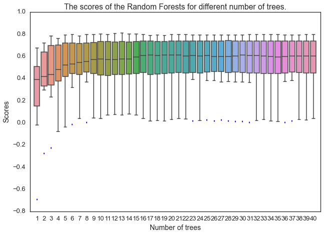
选择树的数目为20。

# 使用最优树数进行预测:
RF_e = RandomForestRegressor(n_estimators=20, max_depth=None, 
                             min_samples_split=1, random_state=0)
RF_e.fit(XX_elect_train,YY_elect_train)
YY_elect_pred=RF_e.predict(XX_elect_test)

fig,ax = plt.subplots(1, 1,figsize=(20,10))
line1, =plt.plot(XX_elect_test.index, YY_elect_test, 
                 label='Actual consumption', color='k')
line2, =plt.plot(XX_elect_test.index, YY_elect_pred, 
                 label='RF Regression Prediction', color='r')
plt.xlabel('Feature index',fontsize=18)
plt.ylabel('Normalized electricity usage (kWh)',fontsize=18)
plt.title('Actual and RF predicted electricity usage',fontsize=20)
plt.legend([line1, line2], ['Actual consumption', 'RF Regression Prediction'],fontsize=18)
plt.show()

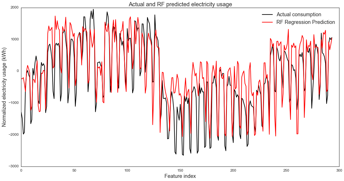
print RF_e.score(XX_elect_test,YY_elect_test)

0.679872383518

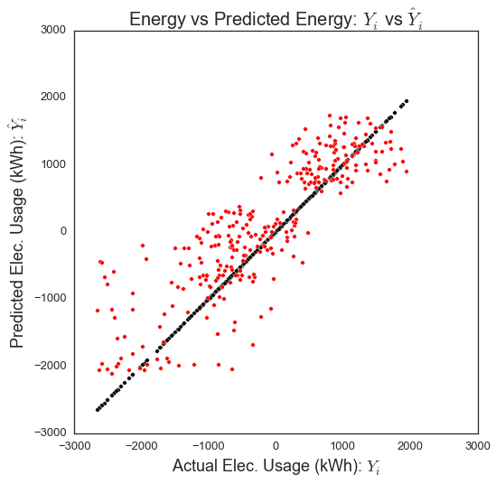
# 展示真实数据和预测数据.
fig = plt.figure(figsize=(8,8))
plt.scatter(YY_elect_test, YY_elect_test, c='k')
plt.scatter(YY_elect_test, YY_elect_pred, c='r')
plt.xlabel('Actual Elec. Usage (kWh): $Y_i$',fontsize=18)
plt.ylabel("Predicted Elec. Usage (kWh): $hat{Y}_i$",fontsize=18)
plt.title("Energy vs Predicted Energy: $Y_i$ vs $hat{Y}_i$",fontsize=20)
plt.show()

分析冷水数据

chilledw_train = pd.DataFrame(data=normalized_chilledWater, 
                              index=np.arange('2012-01', '2014-01',
                                              dtype='datetime64[D]')).dropna()
chilledw_test = pd.DataFrame(data=normalized_chilledWater, 
                             index=np.arange('2014-01', '2014-11', 
                                             dtype='datetime64[D]')).dropna()

XX_chilledw_train = chilledw_train.drop('chilledWater-TonDays', 
                                        axis = 1).reset_index().drop('index', axis = 1)
XX_chilledw_test = chilledw_test.drop('chilledWater-TonDays', 
                                      axis = 1).reset_index().drop('index', axis = 1)

YY_chilledw_train = chilledw_train['chilledWater-TonDays']
YY_chilledw_test = chilledw_test['chilledWater-TonDays']

print XX_chilledw_train.shape, XX_chilledw_test.shape

(705, 13) (294, 13)

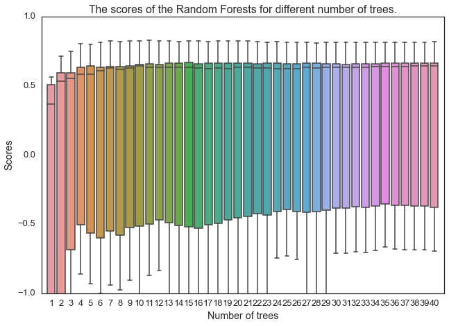
# 找出最佳的树的数目。
scores = pd.DataFrame()
for n in range(1,41):
    rf = RandomForestRegressor(n_estimators=n, max_depth=None, min_samples_split=1, random_state=0)
    score = cross_val_score(rf, XX_chilledw_train, YY_chilledw_train,cv=10)
    scores[n] = score

sns.set_context("talk")
sns.set_style("white")

sns.boxplot(np.matrix(scores))
plt.xlabel("Number of trees")
plt.ylabel("Scores")
plt.title("The scores of the Random Forests for different number of trees.")
plt.xlim(0,41)
plt.ylim(-1,1)
plt.show()

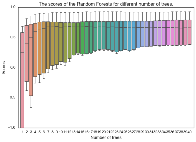
选择树的数目为20。

# 使用最优树数进行预测:
RF_w = RandomForestRegressor(n_estimators=20, max_depth=None, min_samples_split=1, random_state=0)
RF_w.fit(XX_chilledw_train,YY_chilledw_train)
YY_chilledw_pred=RF_w.predict(XX_chilledw_test)

fig,ax = plt.subplots(1, 1,figsize=(20,10))
line1, =plt.plot(XX_chilledw_test.index, 
                 YY_chilledw_test, 
                 label='Actual consumption', 
                 color='k')
line2, =plt.plot(XX_chilledw_test.index, 
                 YY_chilledw_pred, 
                 label='RF Regression Prediction', 
                 color='r')
plt.xlabel('Feature index',fontsize=18)
plt.ylabel('Normalized chilled water usage (t)',fontsize=18)
plt.title('Actual and RF predicted chilled water usage',fontsize=20)
plt.legend([line1, line2], ['Actual consumption', 'RF Regression Prediction'],fontsize=18)
plt.show()

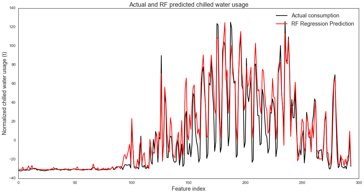
print RF_w.score(XX_chilledw_test,YY_chilledw_test)

0.883316960112

# 绘制实际数据和预测数据。
fig = plt.figure(figsize=(8,8))
plt.scatter(YY_chilledw_test, YY_chilledw_test, c='k')
plt.scatter(YY_chilledw_test, YY_chilledw_pred, c='r')
plt.xlabel('Actual Water Usage (Ton): $Y_i$',fontsize=18)
plt.ylabel("Predicted Water Usage (Ton): $hat{Y}_i$",fontsize=18)
plt.title("Water vs Predicted Water: $Y_i$ vs $hat{Y}_i$",
          fontsize=18)
plt.show()

分析热水数据

steam_train = pd.DataFrame(data=normalized_steam, 
                           index=np.arange('2012-01', '2014-01', 
                                           dtype='datetime64[D]')).dropna()
steam_test = pd.DataFrame(data=normalized_steam, 
                          index=np.arange('2014-01', '2014-11', 
                                          dtype='datetime64[D]')).dropna()

XX_steam_train = steam_train.drop('steam-LBS', axis = 1).reset_index().drop('index', 
                                                                            axis = 1)
XX_steam_test = steam_test.drop('steam-LBS', axis = 1).reset_index().drop('index', 
                                                                          axis = 1)

YY_steam_train = steam_train['steam-LBS']
YY_steam_test = steam_test['steam-LBS']

print XX_steam_train.shape, XX_steam_test.shape

(705, 13) (294, 13)

# 找出最佳的树的数目。
scores = pd.DataFrame()
for n in range(1,41):
    Rf = RandomForestRegressor(n_estimators=n, max_depth=None, 
                               min_samples_split=1, random_state=0)
    score = cross_val_score(Rf, XX_steam_train, YY_steam_train,cv=10)
    scores[n] = score

sns.set_context("talk")
sns.set_style("white")

sns.boxplot(np.matrix(scores))
plt.xlabel("Number of trees")
plt.ylabel("Scores")
plt.title("The scores of the Random Forests for different number of trees.")
plt.xlim(0,41)
plt.ylim(-1,1)
plt.show()

选择树的数目为21。

# 使用最优树数进行预测:
RF_s = RandomForestRegressor(n_estimators=21, max_depth=None, 
                             min_samples_split=1, random_state=0)
RF_s.fit(XX_steam_train,YY_steam_train)
YY_steam_pred=RF_s.predict(XX_steam_test)

fig,ax = plt.subplots(1, 1,figsize=(20,10))
line1, =plt.plot(XX_steam_test.index, YY_steam_test, 
                 label='Actual consumption', color='k')
line2, =plt.plot(XX_steam_test.index, YY_steam_pred, 
                 label='RF Regression Prediction', color='r')
plt.xlabel('Feature index',fontsize=18)
plt.ylabel('Normalized steam usage (LBS)',fontsize=18)
plt.title('Actual and RF predicted steam usage',fontsize=20)
plt.legend([line1, line2], ['Actual consumption', 'RF Regression Prediction'],fontsize=18)
plt.show()

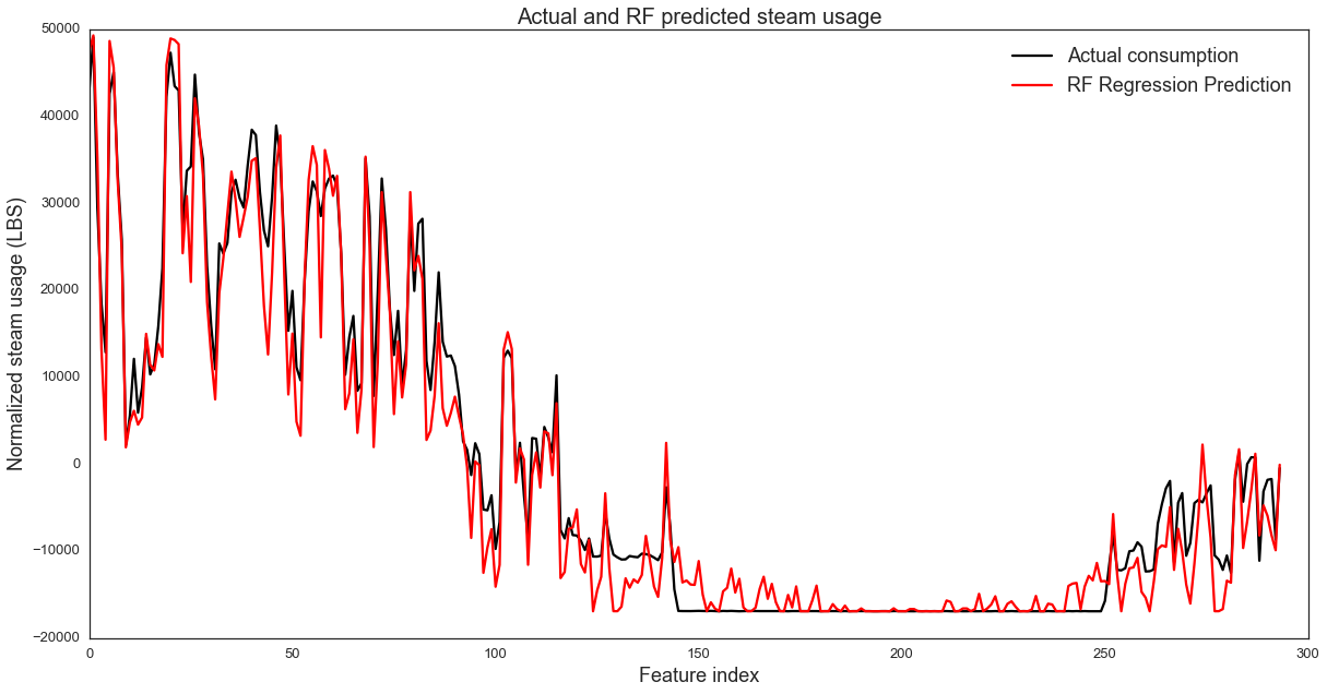
print RF_s.score(XX_steam_test,YY_steam_test)

0.960889669644

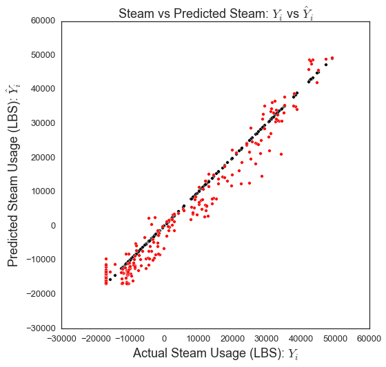
# 绘制实际数据和预测数据。
fig = plt.figure(figsize=(8,8))
plt.scatter(YY_steam_test, YY_steam_test, c='k')
plt.scatter(YY_steam_test, YY_steam_pred, c='r')
plt.xlabel('Actual Steam Usage (LBS): $Y_i$',fontsize=18)
plt.ylabel("Predicted Steam Usage (LBS): $hat{Y}_i$",fontsize=18)
plt.title("Steam vs Predicted Steam: $Y_i$ vs $hat{Y}_i$",fontsize=18)
plt.show()

4.2 K最邻近

在这本笔记本中，我们将训练一个基于历史能源数据和几个天气变量的KNN回归模型来预测建筑能耗。我们将使用每日能源数据和天气数据来预测能源消耗。

%matplotlib inline 
import numpy as np
import pandas as pd

import matplotlib.pyplot as plt

pd.options.display.mpl_style = 'default'

import seaborn as sns 

import sklearn
import sklearn.datasets
import sklearn.cross_validation
import sklearn.decomposition
import sklearn.grid_search
import sklearn.neighbors
import sklearn.metrics

建立KNN回归模型，从平均调整天气属性预测用电量。为此，我们将把模型与2012年01月01日的每日电力数据和天气数据进行拟合，并计算预测的平均残差平方。

# 读取原始数据:
electricity = pd.read_excel('Data/dailyElectricityWithFeatures.xlsx')
electricity = electricity.drop('startDay', 1).drop('endDay', 1)
#electricity = electricity.drop('humidityRatio-kg/kg',1).drop('coolingDegrees',1).drop('heatingDegrees',1).drop('dehumidification',1).drop('occupancy',1)
electricity = electricity.dropna()

chilledWater = pd.read_excel('Data/dailyChilledWaterWithFeatures.xlsx')
chilledWater = chilledWater.drop('startDay', 1).drop('endDay', 1)
chilledWater = chilledWater.dropna()

steam = pd.read_excel('Data/dailySteamWithFeatures.xlsx')
steam = steam.drop('startDay', 1).drop('endDay', 1)
steam = steam.dropna()

# 规范化数据:
normalized_electricity = electricity - electricity.mean()
normalized_chilledWater = chilledWater - chilledWater.mean()
normalized_steam = steam - steam.mean()

添加一个新列来指定是工作日还是周末和假期。我们将把工作日设为0，把周末和假期设为1。这里列出了美国的公共假期，http://www.officeholidays.com/es/usa/我们也可以在没有学校的情况下取消假期，但是我们会这样做，因为我们没有这些信息。

#初始化天数为0
normalized_electricity['day_type'] = np.zeros(len(normalized_electricity))
normalized_chilledWater['day_type'] = np.zeros(len(normalized_chilledWater))
normalized_steam['day_type'] = np.zeros(len(normalized_steam))

# #初始化周末为0
normalized_electricity['day_type']
					  [(normalized_electricity.index.dayofweek==5)|
			 		   (normalized_electricity.index.dayofweek==6)] = 1
normalized_chilledWater['day_type']
					   [(normalized_chilledWater.index.dayofweek==5)|				
                        (normalized_chilledWater.index.dayofweek==6)] = 1
normalized_steam['day_type'][(normalized_steam.index.dayofweek==5)|(normalized_steam.index.dayofweek==6)] = 1

# #初始化假期为0
holidays = ['2014-01-01','2014-01-20','2014-05-26','2014-07-04','2014-09-01',
            '2014-11-11','2014-11-27','2014-12-25','2013-01-01',
            '2013-01-21','2013-05-27','2013-07-04','2013-09-02','2013-11-11',
            '2013-11-27','2013-12-25','2012-01-01','2012-01-16','2012-05-28',
            '2012-07-04','2012-09-03','2012-11-12','2012-11-22','2012-12-25']

for i in range(len(holidays)):
    normalized_electricity['day_type']
    [normalized_electricity.index.date==np.datetime64(holidays[i])] = 1
    normalized_chilledWater['day_type']
    [normalized_chilledWater.index.date==np.datetime64(holidays[i])] = 1
    normalized_steam['day_type']
    [normalized_steam.index.date==np.datetime64(holidays[i])] = 1

用电数据分析

# 分割训练和测试数据:
elect_train = pd.DataFrame(data=normalized_electricity, 
                           index=np.arange('2012-01', '2014-01',
                                           dtype='datetime64[D]')).dropna()
elect_test = pd.DataFrame(data=normalized_electricity, 
                          index=np.arange('2014-01', '2014-11', 
                                          dtype='datetime64[D]')).dropna()

XX_elect_train = elect_train.drop('electricity-kWh', 
                                  axis = 1).reset_index().drop('index', axis = 1)
XX_elect_test = elect_test.drop('electricity-kWh', 
                                axis = 1).reset_index().drop('index', axis = 1)

YY_elect_train = elect_train['electricity-kWh']
YY_elect_test = elect_test['electricity-kWh']

print XX_elect_train.shape, XX_elect_test.shape

(634, 13) (294, 13)

def accuracy_for_k(k,x,y):
    split_data=sklearn.cross_validation.train_test_split(x,y,test_size=0.33,random_state=99)
    X_train,X_test,Y_train,Y_test=split_data
    knn=sklearn.neighbors.KNeighborsRegressor(n_neighbors=k,weights='uniform')
    knn.fit(X_train,Y_train)
    #Y_hat=knn.predict(X_test)
    value=knn.score(X_test,Y_test)
    return value

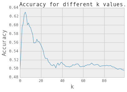
# 求出knn中k的最优数:
k_values=range(1,101)
scores=np.zeros(len(k_values))
for k, c_k in zip(k_values,range(len(k_values))):
    value=accuracy_for_k(k=k,x=XX_elect_train,y=YY_elect_train)
    scores[c_k]=value
    
k_opt=np.argmax(scores)+1
print scores.max()
print 'The optimal value of k is:',k_opt

sns.tsplot(scores.T)
#plt.xticks(range(len(k_values)),k_values)
plt.xlabel('k',fontsize=18)
plt.ylabel('Accuracy',fontsize=18)
plt.title('Accuracy for different k values.',fontsize=18)
plt.show()

0.0305837055412
The optimal value of k is: 30

# 用最优k预测:
knn_reg=sklearn.neighbors.KNeighborsRegressor(n_neighbors=31,weights='uniform')
knn_reg.fit(XX_elect_train,YY_elect_train)
YY_elect_pred=knn_reg.predict(XX_elect_test)

fig,ax = plt.subplots(1, 1,figsize=(20,10))
line1, =plt.plot(XX_elect_test.index, YY_elect_test, 
                 label='Actual consumption', color='k')
line2, =plt.plot(XX_elect_test.index, YY_elect_pred, 
                 label='KNN Regression Prediction', color='r')
plt.xlabel('Feature index',fontsize=18)
plt.ylabel('Normalized electricity usage (kWh)',fontsize=18)
plt.title('Actual and KNN predicted electricity usage',fontsize=20)
plt.legend([line1, line2], ['Actual consumption', 
                            'KNN Regression Prediction'],fontsize=18)
plt.show()

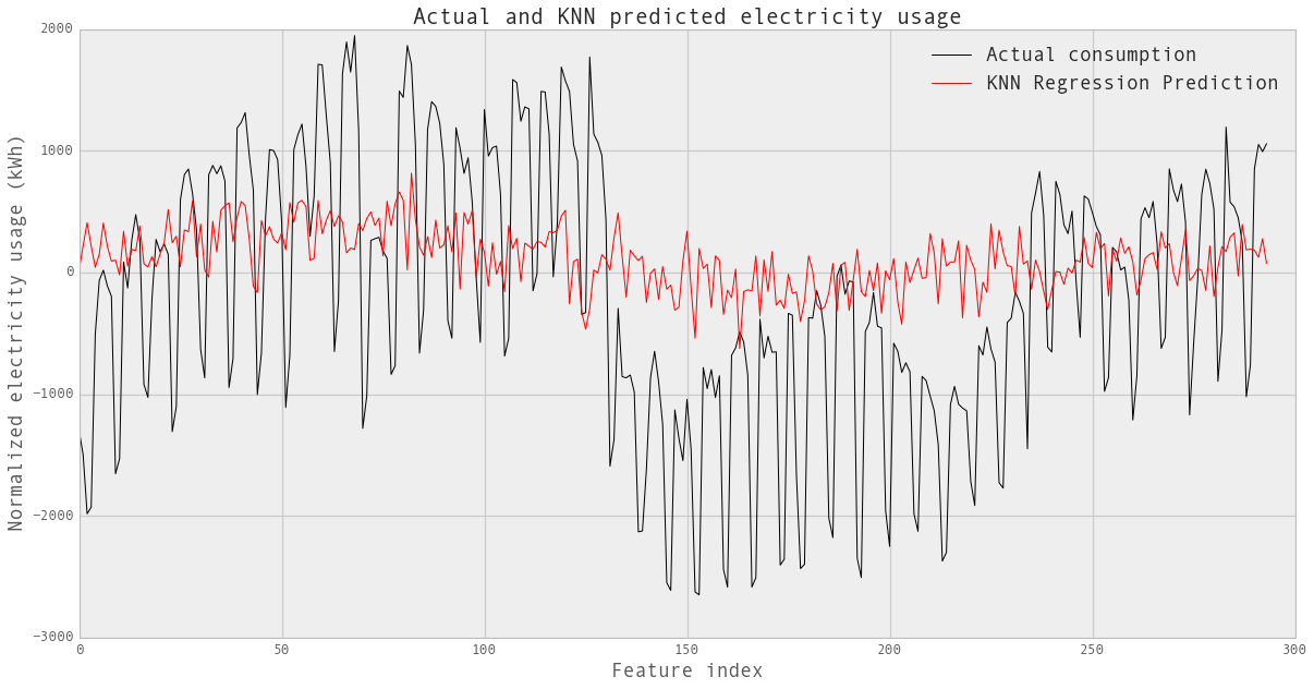
print knn_reg.score(XX_elect_test,YY_elect_test)

0.0450538207392

# 绘制实际数据和预测数据。
fig = plt.figure(figsize=(8,8))
plt.scatter(YY_elect_test, YY_elect_test, c='k')
plt.scatter(YY_elect_test, YY_elect_pred, c='r')
plt.xlabel('Actual Elec. Usage (kWh): $Y_i$',fontsize=18)
plt.ylabel("Predicted Elec. Usage (kWh): $hat{Y}_i$",fontsize=18)

plt.title("Energy vs Predicted Energy: $Y_i$ vs $hat{Y}_i$",fontsize=20)
plt.show()

冷水数据分析。

chilledw_train = pd.DataFrame(data=normalized_chilledWater,
                              index=np.arange('2012-01', '2014-01', 
                                              dtype='datetime64[D]')).dropna()
chilledw_test = pd.DataFrame(data=normalized_chilledWater, 
                             index=np.arange('2014-01', '2014-11', 
                                             dtype='datetime64[D]')).dropna()

XX_chilledw_train = chilledw_train.drop('chilledWater-TonDays', 
                                        axis = 1).reset_index().drop('index', axis = 1)
XX_chilledw_test = chilledw_test.drop('chilledWater-TonDays', 
                                      axis = 1).reset_index().drop('index', axis = 1)

YY_chilledw_train = chilledw_train['chilledWater-TonDays']
YY_chilledw_test = chilledw_test['chilledWater-TonDays']

print XX_chilledw_train.shape, XX_chilledw_test.shape

(705, 13) (294, 13)

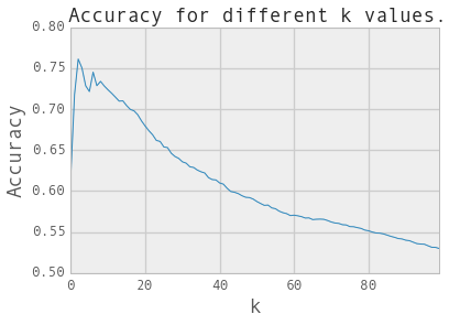
# 求出knn中k的最优个数:
k_values=range(1,101)
scores=np.zeros(len(k_values))
for k, c_k in zip(k_values,range(len(k_values))):
    value=accuracy_for_k(k=k,x=XX_chilledw_train,y=YY_chilledw_train)
    scores[c_k]=value
    
k_opt=np.argmax(scores)+1
print scores.max()
print 'The optimal value of k is:',k_opt

sns.tsplot(scores.T)
#plt.xticks(range(len(k_values)),k_values)
plt.xlabel('k',fontsize=18)
plt.ylabel('Accuracy',fontsize=18)
plt.title('Accuracy for different k values.',fontsize=18)
plt.show()

0.62985747618
The optimal value of k is: 6

# 用最优k预测:
knn_reg_w=sklearn.neighbors.KNeighborsRegressor(n_neighbors=6,weights='uniform')
knn_reg_w.fit(XX_chilledw_train,YY_chilledw_train)
YY_chilledw_pred=knn_reg_w.predict(XX_chilledw_test)

fig,ax = plt.subplots(1, 1,figsize=(20,10))
line1, =plt.plot(XX_chilledw_test.index, YY_chilledw_test, 
                 label='Actual consumption', color='k')
line2, =plt.plot(XX_chilledw_test.index, YY_chilledw_pred, 
                 label='KNN Regression Prediction', color='r')
plt.xlabel('Feature index',fontsize=18)
plt.ylabel('Normalized chilled water usage (t)',fontsize=18)
plt.title('Actual and KNN predicted chilled water usage',fontsize=20)
plt.legend([line1, line2], ['Actual consumption', 'KNN Regression Prediction'],fontsize=18)
plt.show()

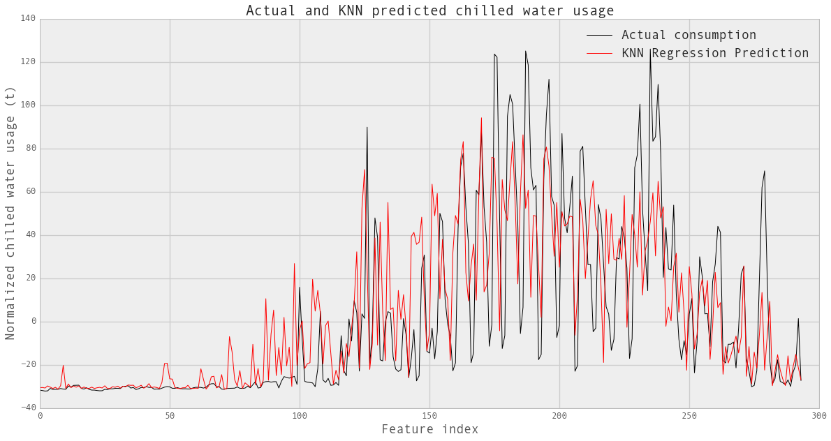
print knn_reg_w.score(XX_chilledw_test,YY_chilledw_test)

0.50450369365

#Plot actual vs. prediced usage.
fig = plt.figure(figsize=(8,8))
plt.scatter(YY_chilledw_test, YY_chilledw_test, c='k')
plt.scatter(YY_chilledw_test, YY_chilledw_pred, c='r')
plt.xlabel('Actual Water Usage (Ton): $Y_i$',fontsize=18)
plt.ylabel("Predicted Water Usage (Ton): $hat{Y}_i$",fontsize=18)
plt.title("Water vs Predicted Water: $Y_i$ vs $hat{Y}_i$",fontsize=18)
plt.show()

热水数据分析

steam_train = pd.DataFrame(data=normalized_steam, 
                           index=np.arange('2012-01', '2014-01', dtype='datetime64[D]')).dropna()
steam_test = pd.DataFrame(data=normalized_steam, 
                          index=np.arange('2014-01', '2014-11', dtype='datetime64[D]')).dropna()

XX_steam_train = steam_train.drop('steam-LBS', 
                                  axis = 1).reset_index().drop('index', axis = 1)
XX_steam_test = steam_test.drop('steam-LBS', 
                                axis = 1).reset_index().drop('index', axis = 1)

YY_steam_train = steam_train['steam-LBS']
YY_steam_test = steam_test['steam-LBS']

print XX_steam_train.shape, XX_steam_test.shape

(705, 13) (294, 13)

# 求出knn中k的最优个数:
k_values=range(1,101)
scores=np.zeros(len(k_values))
for k, c_k in zip(k_values,range(len(k_values))):
    value=accuracy_for_k(k=k,x=XX_steam_train,y=YY_steam_train)
    scores[c_k]=value
    
k_opt=np.argmax(scores)+1
print scores.max()
print 'The optimal value of k is:',k_opt

sns.tsplot(scores.T)
#plt.xticks(range(len(k_values)),k_values)
plt.xlabel('k',fontsize=18)
plt.ylabel('Accuracy',fontsize=18)
plt.title('Accuracy for different k values.',fontsize=18)
plt.show()

0.760976988296
The optimal value of k is: 3

# 用最优k预测:
knn_reg_s=sklearn.neighbors.KNeighborsRegressor(n_neighbors=3,weights='uniform')
knn_reg_s.fit(XX_steam_train,YY_steam_train)
YY_steam_pred=knn_reg_s.predict(XX_steam_test)

fig,ax = plt.subplots(1, 1,figsize=(20,10))
line1, =plt.plot(XX_steam_test.index, 
                 YY_steam_test, label='Actual consumption', color='k')
line2, =plt.plot(XX_steam_test.index, 
                 YY_steam_pred, label='KNN Regression Prediction', color='r')
plt.xlabel('Feature index',fontsize=18)
plt.ylabel('Normalized steam usage (LBS)',fontsize=18)
plt.title('Actual and KNN predicted steam usage',fontsize=20)
plt.legend([line1, line2], ['Actual consumption', 'KNN Regression Prediction'],fontsize=18)
plt.show()

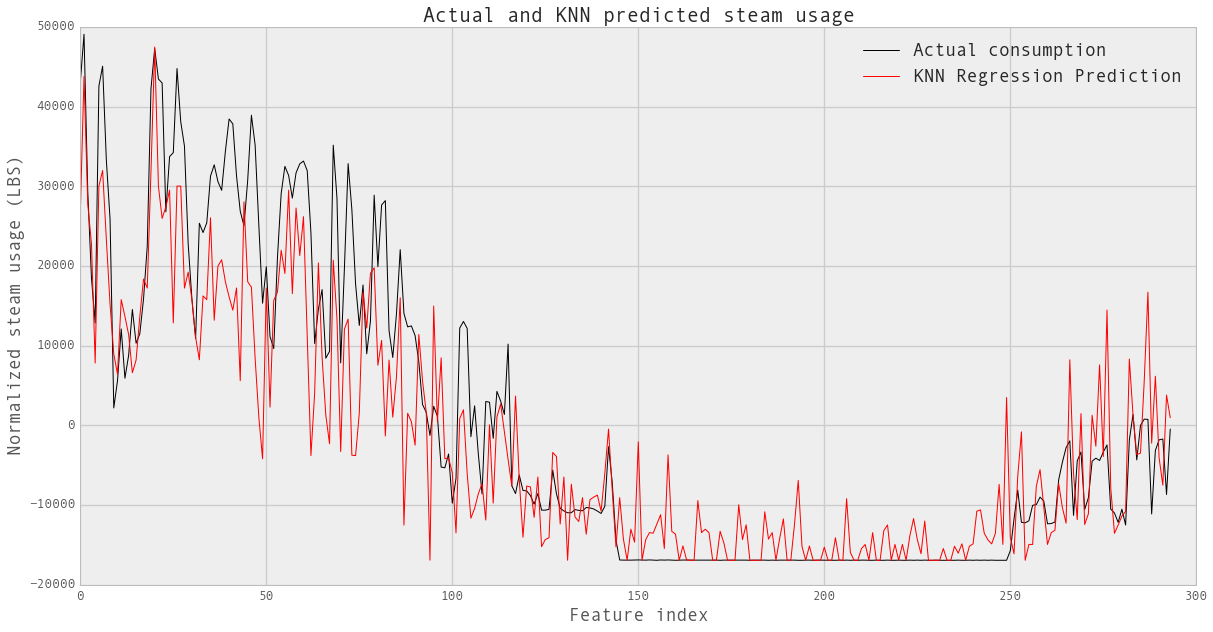
print knn_reg_s.score(XX_steam_test,YY_steam_test)

0.787718743908

# 绘制实际数据和预测数据。
fig = plt.figure(figsize=(8,8))
plt.scatter(YY_steam_test/10000, YY_steam_test/10000, c='k')
plt.scatter(YY_steam_test/10000, YY_steam_pred/10000, c='r')
plt.xlabel('Actual Steam Usage ($10^4$LBS): $Y_i$',fontsize=16)
plt.ylabel("Predicted Steam Usage ($10^4$LBS): $hat{Y}_i$",fontsize=18)
plt.title("Steam vs Predicted Steam: $Y_i$ vs $hat{Y}_i$",fontsize=18)
plt.show()

下篇5_Summary, Conclusion and Discussion