损失函数:
求解结果:
1、读取数据
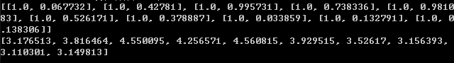
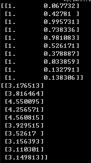
部分数据如下
1.000000    0.067732    3.176513
1.000000    0.427810    3.816464
1.000000    0.995731    4.550095
1.000000    0.738336    4.256571
1.000000    0.981083    4.560815
1.000000    0.526171    3.929515
1.000000    0.378887    3.526170
1.000000    0.033859    3.156393
1.000000    0.132791    3.110301
1.000000    0.138306    3.149813
python代码:
from numpy import *
import numpy as np

def loadDataSet(fileName):      #general function to parse tab -delimited floats
    numFeat = len(open(fileName).readline().split('	')) - 1 #get number of fields
    dataMat = []
    labelMat = []
    fr = open(fileName)
    for line in fr.readlines():
        lineArr =[]
        curLine = line.strip().split('	')
        for i in range(numFeat):
            lineArr.append(float(curLine[i]))
        dataMat.append(lineArr)
        labelMat.append(float(curLine[-1]))
    return dataMat,labelMat
xArr,yArr=loadDataSet("ex0.txt")
部分结果:
需要注意的是xArr中的第一项均为1,其实是偏置项的占位。我们要想可视化数据的分布,在读取数据的时候可以不用考虑:
def loadDataSet2(fileName):      #general function to parse tab -delimited floats
    numFeat = len(open(fileName).readline().split('	')) - 1 #get number of fields
    dataMat = []
    labelMat = []
    fr = open(fileName)
    for line in fr.readlines():
        curLine = line.strip().split('	')
        for i in range(1,numFeat):
            dataMat.append(float(curLine[i]))
        labelMat.append(float(curLine[-1]))
    return dataMat,labelMat
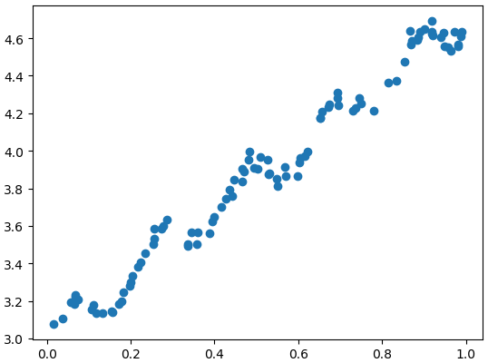
然后绘制散点图:
xArr2, yArr2 = loadDataSet2('ex0.txt')
plt.plot(xArr2[100:199],yArr2[100:199],'o')
plt.show()
结果:
2、定义损失函数
def rssError(yArr,yHatArr): #yArr and yHatArr both need to be arrays
    return ((yArr-yHatArr)**2).sum()
3、简单线性回归
def standRegres(xArr,yArr):
    xMat=mat(xArr)
    yMat=mat(yArr).T
    print(xMat[:10])
    print(yMat[:10])
    xTx = xMat.T*xMat
    if linalg.det(xTx) == 0.0:
        print("This matrix is singular, cannot do inverse")
        return
    ws = xTx.I * (xMat.T*yMat)
    return ws
xMat和yMat的部分结果:
4、开始执行
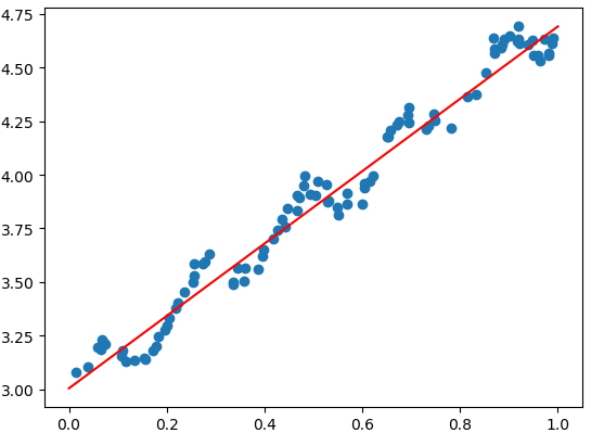
我们利用前100个数据计算出ws,然后利用后100个数据进行预测:
if __name__ == "__main__"    :

    xArr, yArr = loadDataSet('ex0.txt')
    ws = standRegres(xArr[0:99], yArr[0:99])
    print(ws)

    yHat = mat(xArr[100:199]) * ws
    #计算损失
    print(rssError(yArr[100:199],yHat.T.A))
    #将输入限制在0-1之间
    x_test=np.array([[0],[1]])
    #计算结果
    y_test=ws[0]+x_test*ws[1]

    #画出曲线
    xArr2, yArr2 = loadDataSet2('ex0.txt')
    plt.plot(xArr2[100:199],yArr2[100:199],'o')
    plt.plot(x_test,y_test,'r')
    plt.show()
最后的结果是这样的:
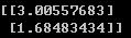
ws的值:
损失:

可视化结果: