python实现多层感知机

什么是多层感知机？

多层感知机（MLP，Multilayer Perceptron）也叫人工神经网络（ANN，Artificial Neural Network），除了输入输出层，它中间可以有多个隐层，最简单的MLP只含一个隐层，即三层的结构，如下图：

上图可以看到，多层感知机层与层之间是全连接的。多层感知机最底层是输入层，中间是隐藏层，最后是输出层。 

参考：https://blog.csdn.net/fg13821267836/article/details/93405572 

多层感知机和感知机的区别？

我们来看下感知机是什么样的：

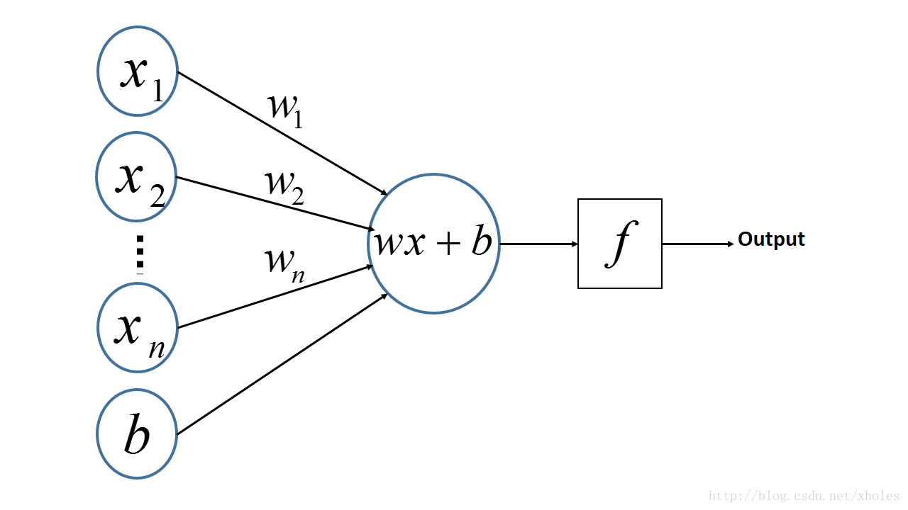
从上述内容更可以看出，感知机是一个线性的二分类器，但不能对非线性的数据并不能进行有效的分类。因此便有了对网络层次的加深，理论上，多层感知机可以模拟任何复杂的函数。 

多层感知机的前向传播过程？

这里以输入层、一个隐含层，输出层为例：

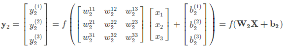
结合之前定义的字母标记，对于第二层的三个神经元的输出则有： 

将上述的式子转换为矩阵表达式：

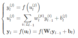
将第二层的前向传播计算过程推广到网络中的任意一层，则:

多层感知机的反向传播过程？

可参考：https://blog.csdn.net/xholes/article/details/78461164 

下面是实现代码：代码来源：https://github.com/eriklindernoren/ML-From-Scratch 

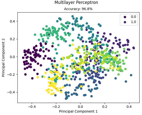
from __future__ import print_function, division
import numpy as np
import math
from sklearn import datasets

from mlfromscratch.utils import train_test_split, to_categorical, normalize, accuracy_score, Plot
from mlfromscratch.deep_learning.activation_functions import Sigmoid, Softmax
from mlfromscratch.deep_learning.loss_functions import CrossEntropy

class MultilayerPerceptron():
    """Multilayer Perceptron classifier. A fully-connected neural network with one hidden layer.
    Unrolled to display the whole forward and backward pass.

    Parameters:
    -----------
    n_hidden: int:
        The number of processing nodes (neurons) in the hidden layer. 
    n_iterations: float
        The number of training iterations the algorithm will tune the weights for.
    learning_rate: float
        The step length that will be used when updating the weights.
    """
    def __init__(self, n_hidden, n_iterations=3000, learning_rate=0.01):
        self.n_hidden = n_hidden
        self.n_iterations = n_iterations
        self.learning_rate = learning_rate
        self.hidden_activation = Sigmoid()
        self.output_activation = Softmax()
        self.loss = CrossEntropy()

    def _initialize_weights(self, X, y):
        n_samples, n_features = X.shape
        _, n_outputs = y.shape
        # Hidden layer
        limit   = 1 / math.sqrt(n_features)
        self.W  = np.random.uniform(-limit, limit, (n_features, self.n_hidden))
        self.w0 = np.zeros((1, self.n_hidden))
        # Output layer
        limit   = 1 / math.sqrt(self.n_hidden)
        self.V  = np.random.uniform(-limit, limit, (self.n_hidden, n_outputs))
        self.v0 = np.zeros((1, n_outputs))

    def fit(self, X, y):

        self._initialize_weights(X, y)

        for i in range(self.n_iterations):

            # ..............
            #  Forward Pass
            # ..............

            # HIDDEN LAYER
            hidden_input = X.dot(self.W) + self.w0
            hidden_output = self.hidden_activation(hidden_input)
            # OUTPUT LAYER
            output_layer_input = hidden_output.dot(self.V) + self.v0
            y_pred = self.output_activation(output_layer_input)

            # ...............
            #  Backward Pass
            # ...............

            # OUTPUT LAYER
            # Grad. w.r.t input of output layer
            grad_wrt_out_l_input = self.loss.gradient(y, y_pred) * self.output_activation.gradient(output_layer_input)
            grad_v = hidden_output.T.dot(grad_wrt_out_l_input)
            grad_v0 = np.sum(grad_wrt_out_l_input, axis=0, keepdims=True)
            # HIDDEN LAYER
            # Grad. w.r.t input of hidden layer
            grad_wrt_hidden_l_input = grad_wrt_out_l_input.dot(self.V.T) * self.hidden_activation.gradient(hidden_input)
            grad_w = X.T.dot(grad_wrt_hidden_l_input)
            grad_w0 = np.sum(grad_wrt_hidden_l_input, axis=0, keepdims=True)

            # Update weights (by gradient descent)
            # Move against the gradient to minimize loss
            self.V  -= self.learning_rate * grad_v
            self.v0 -= self.learning_rate * grad_v0
            self.W  -= self.learning_rate * grad_w
            self.w0 -= self.learning_rate * grad_w0

    # Use the trained model to predict labels of X
    def predict(self, X):
        # Forward pass:
        hidden_input = X.dot(self.W) + self.w0
        hidden_output = self.hidden_activation(hidden_input)
        output_layer_input = hidden_output.dot(self.V) + self.v0
        y_pred = self.output_activation(output_layer_input)
        return y_pred


def main():
    data = datasets.load_digits()
    X = normalize(data.data)
    y = data.target

    # Convert the nominal y values to binary
    y = to_categorical(y)

    X_train, X_test, y_train, y_test = train_test_split(X, y, test_size=0.4, seed=1)

    # MLP
    clf = MultilayerPerceptron(n_hidden=16,
        n_iterations=1000,
        learning_rate=0.01)

    clf.fit(X_train, y_train)
    y_pred = np.argmax(clf.predict(X_test), axis=1)
    y_test = np.argmax(y_test, axis=1)

    accuracy = accuracy_score(y_test, y_pred)
    print ("Accuracy:", accuracy)

    # Reduce dimension to two using PCA and plot the results
    Plot().plot_in_2d(X_test, y_pred, title="Multilayer Perceptron", accuracy=accuracy, legend_labels=np.unique(y))

if __name__ == "__main__":
    main()

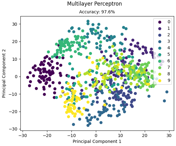
运行结果：

Accuracy: 0.967966573816156

另外的一种实现是使用卷积神经网络中的全连接层实现：

from __future__ import print_function
from sklearn import datasets
import matplotlib.pyplot as plt
import numpy as np
import sys
sys.path.append("/content/drive/My Drive/learn/ML-From-Scratch/")
# Import helper functions
from mlfromscratch.deep_learning import NeuralNetwork
from mlfromscratch.utils import train_test_split, to_categorical, normalize, Plot
from mlfromscratch.utils import get_random_subsets, shuffle_data, accuracy_score
from mlfromscratch.deep_learning.optimizers import StochasticGradientDescent, Adam, RMSprop, Adagrad, Adadelta
from mlfromscratch.deep_learning.loss_functions import CrossEntropy
from mlfromscratch.utils.misc import bar_widgets
from mlfromscratch.deep_learning.layers import Dense, Dropout, Activation


def main():

    optimizer = Adam()

    #-----
    # MLP
    #-----

    data = datasets.load_digits()
    X = data.data
    y = data.target

    # Convert to one-hot encoding
    y = to_categorical(y.astype("int"))

    n_samples, n_features = X.shape
    n_hidden = 512

    X_train, X_test, y_train, y_test = train_test_split(X, y, test_size=0.4, seed=1)

    clf = NeuralNetwork(optimizer=optimizer,
                        loss=CrossEntropy,
                        validation_data=(X_test, y_test))

    clf.add(Dense(n_hidden, input_shape=(n_features,)))
    clf.add(Activation('leaky_relu'))
    clf.add(Dense(n_hidden))
    clf.add(Activation('leaky_relu'))
    clf.add(Dropout(0.25))
    clf.add(Dense(n_hidden))
    clf.add(Activation('leaky_relu'))
    clf.add(Dropout(0.25))
    clf.add(Dense(n_hidden))
    clf.add(Activation('leaky_relu'))
    clf.add(Dropout(0.25))
    clf.add(Dense(10))
    clf.add(Activation('softmax'))

    print ()
    clf.summary(name="MLP")
    
    train_err, val_err = clf.fit(X_train, y_train, n_epochs=50, batch_size=256)
    
    # Training and validation error plot
    n = len(train_err)
    training, = plt.plot(range(n), train_err, label="Training Error")
    validation, = plt.plot(range(n), val_err, label="Validation Error")
    plt.legend(handles=[training, validation])
    plt.title("Error Plot")
    plt.ylabel('Error')
    plt.xlabel('Iterations')
    plt.show()

    _, accuracy = clf.test_on_batch(X_test, y_test)
    print ("Accuracy:", accuracy)

    # Reduce dimension to 2D using PCA and plot the results
    y_pred = np.argmax(clf.predict(X_test), axis=1)
    Plot().plot_in_2d(X_test, y_pred, title="Multilayer Perceptron", accuracy=accuracy, legend_labels=range(10))


if __name__ == "__main__":
    main()

运行结果：

+-----+
| MLP |
+-----+
Input Shape: (64,)
+------------------------+------------+--------------+
| Layer Type             | Parameters | Output Shape |
+------------------------+------------+--------------+
| Dense                  | 33280      | (512,)       |
| Activation (LeakyReLU) | 0          | (512,)       |
| Dense                  | 262656     | (512,)       |
| Activation (LeakyReLU) | 0          | (512,)       |
| Dropout                | 0          | (512,)       |
| Dense                  | 262656     | (512,)       |
| Activation (LeakyReLU) | 0          | (512,)       |
| Dropout                | 0          | (512,)       |
| Dense                  | 262656     | (512,)       |
| Activation (LeakyReLU) | 0          | (512,)       |
| Dropout                | 0          | (512,)       |
| Dense                  | 5130       | (10,)        |
| Activation (Softmax)   | 0          | (10,)        |
+------------------------+------------+--------------+
Total Parameters: 826378

Training: 100% [------------------------------------------------] Time:  0:00:29

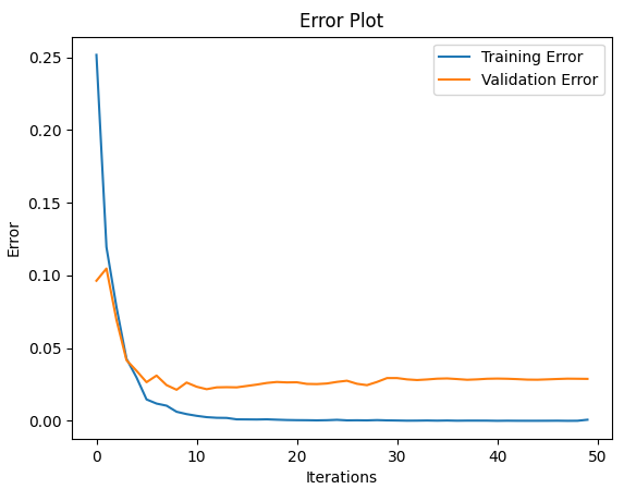
Accuracy: 0.9763231197771588