谱聚类的python实现

什么是谱聚类？

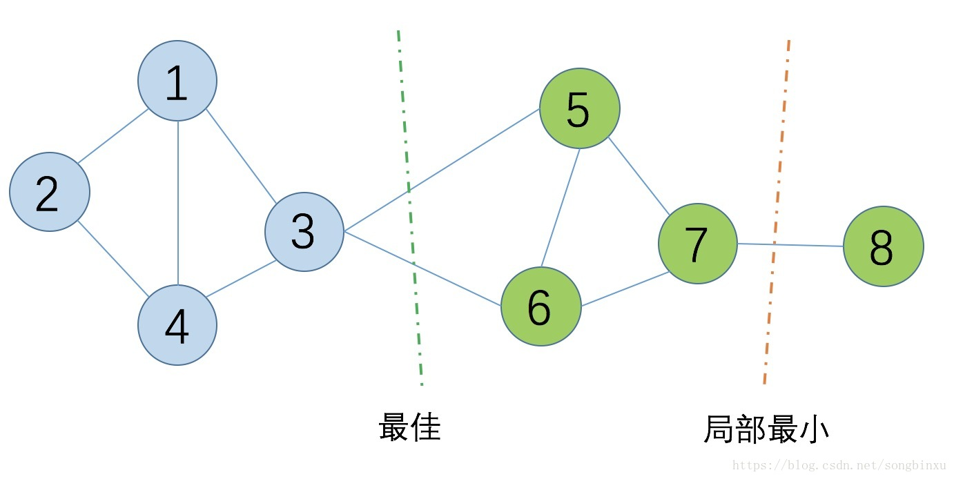
就是找到一个合适的切割点将图进行切割，核心思想就是：

使得切割的边的权重和最小，对于无向图而言就是切割的边数最少，如上所示。但是，切割的时候可能会存在局部最优，有以下两种方法：

（1）RatioCut：核心是要求划分出来的子图的节点数尽可能的大

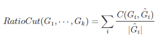
分母变为子图的节点的个数 。

（2）NCut：考虑每个子图的边的权重和

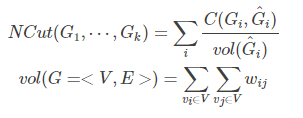
分母变为子图各边的权重和。

具体之后求解可以参考：https://blog.csdn.net/songbinxu/article/details/80838865 

谱聚类的整体流程？

1. 计算距离矩阵（例如欧氏距离）
2. 利用KNN计算邻接矩阵 A
   
3. 由 A 计算度矩阵 D 和拉普拉斯矩阵 L
   
4. 标准化 L→$D^{−1/2}LD^{−1/2}$
5. 对矩阵 $D^{−1/2}LD^{−1/2}$进行特征值分解，得到特征向量 $H_{nn}$
   
6. 将  $H_{nn}$ 当成样本送入 Kmeans 聚类
7. 获得聚类结果 C=(C1,C2,⋯,Ck)

python实现：

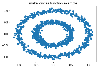
（1）首先是数据的生成：

from sklearn import datasets

  x1, y1 = datasets.make_circles(n_samples=1000, factor=0.5, noise=0.05)

import matplotlib.pyplot as plt
%matplotlib inline
plt.title('make_circles function example')
plt.scatter(x1[:, 0], x1[:, 1], marker='o')
plt.show()

x1的形状是(1000,2)

（2）接下来，我们要计算两两样本之间的距离：

import numpy as np
def euclidDistance(x1, x2, sqrt_flag=False):
    res = np.sum((x1-x2)**2)
    if sqrt_flag:
        res = np.sqrt(res)
    return res

将这些距离用矩阵的形式保存：

def calEuclidDistanceMatrix(X):
    X = np.array(X)
    S = np.zeros((len(X), len(X)))
    for i in range(len(X)):
        for j in range(i+1, len(X)):
            S[i][j] = 1.0 * euclidDistance(X[i], X[j])
            S[j][i] = S[i][j]
    return S

S = calEuclidDistanceMatrix(x1)

array([[0.00000000e+00, 1.13270081e+00, 2.62565479e+00, ...,
        2.99144277e+00, 1.88193070e+00, 1.12840739e+00],
       [1.13270081e+00, 0.00000000e+00, 2.72601994e+00, ...,
        2.95125426e+00, 5.11864947e-01, 6.05388856e-05],
       [2.62565479e+00, 2.72601994e+00, 0.00000000e+00, ...,
        1.30747922e-02, 1.18180915e+00, 2.74692378e+00],
       ...,
       [2.99144277e+00, 2.95125426e+00, 1.30747922e-02, ...,
        0.00000000e+00, 1.26037239e+00, 2.97382982e+00],
       [1.88193070e+00, 5.11864947e-01, 1.18180915e+00, ...,
        1.26037239e+00, 0.00000000e+00, 5.22992113e-01],
       [1.12840739e+00, 6.05388856e-05, 2.74692378e+00, ...,
        2.97382982e+00, 5.22992113e-01, 0.00000000e+00]])

（3）使用KNN计算跟每个样本最接近的k个样本点，然后计算出邻接矩阵：

def myKNN(S, k, sigma=1.0):
    N = len(S)
    #定义邻接矩阵
    A = np.zeros((N,N))
    for i in range(N):
        #对每个样本进行编号
        dist_with_index = zip(S[i], range(N))
        #对距离进行排序
        dist_with_index = sorted(dist_with_index, key=lambda x:x[0])
        #取得距离该样本前k个最小距离的编号
        neighbours_id = [dist_with_index[m][1] for m in range(k+1)] # xi's k nearest neighbours
        #构建邻接矩阵
        for j in neighbours_id: # xj is xi's neighbour
            A[i][j] = np.exp(-S[i][j]/2/sigma/sigma)
            A[j][i] = A[i][j] # mutually

    return A

A = myKNN(S,3)

array([[1.        , 0.        , 0.        , ..., 0.        , 0.        ,
        0.        ],
       [0.        , 1.        , 0.        , ..., 0.        , 0.        ,
        0.99996973],
       [0.        , 0.        , 1.        , ..., 0.        , 0.        ,
        0.        ],
       ...,
       [0.        , 0.        , 0.        , ..., 1.        , 0.        ,
        0.        ],
       [0.        , 0.        , 0.        , ..., 0.        , 1.        ,
        0.        ],
       [0.        , 0.99996973, 0.        , ..., 0.        , 0.        ,
        1.        ]])

（4）计算标准化的拉普拉斯矩阵

def calLaplacianMatrix(adjacentMatrix):

    # compute the Degree Matrix: D=sum(A)
    degreeMatrix = np.sum(adjacentMatrix, axis=1)

    # compute the Laplacian Matrix: L=D-A
    laplacianMatrix = np.diag(degreeMatrix) - adjacentMatrix

    # normailze
    # D^(-1/2) L D^(-1/2)
    sqrtDegreeMatrix = np.diag(1.0 / (degreeMatrix ** (0.5)))
    return np.dot(np.dot(sqrtDegreeMatrix, laplacianMatrix), sqrtDegreeMatrix)

L_sys = calLaplacianMatrix(A)

array([[ 0.66601736,  0.        ,  0.        , ...,  0.        ,
         0.        ,  0.        ],
       [ 0.        ,  0.74997723,  0.        , ...,  0.        ,
         0.        , -0.28868642],
       [ 0.        ,  0.        ,  0.74983185, ...,  0.        ,
         0.        ,  0.        ],
       ...,
       [ 0.        ,  0.        ,  0.        , ...,  0.66662382,
         0.        ,  0.        ],
       [ 0.        ,  0.        ,  0.        , ...,  0.        ,
         0.74953329,  0.        ],
       [ 0.        , -0.28868642,  0.        , ...,  0.        ,
         0.        ,  0.66665079]])

（5）特征值分解

lam, V = np.linalg.eig(L_sys) # H'shape is n*n
lam = zip(lam, range(len(lam)))
lam = sorted(lam, key=lambda x:x[0])
H = np.vstack([V[:,i] for (v, i) in lam[:1000]]).T
H = np.asarray(H).astype(float)

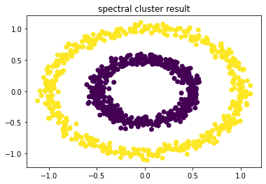
（6）使用谱聚类进行聚类

from sklearn.cluster import KMeans
def spKmeans(H):
    sp_kmeans = KMeans(n_clusters=2).fit(H)
    return sp_kmeans.labels_

labels = spKmeans(H)
plt.title('spectral cluster result')
plt.scatter(x1[:, 0], x1[:, 1], marker='o',c=labels)
plt.show()

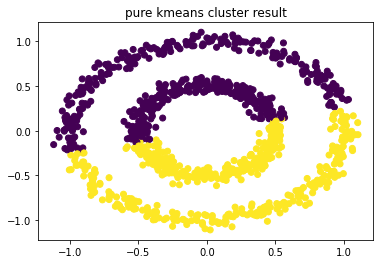
（7） 对比使用kmeans聚类

pure_kmeans = KMeans(n_clusters=2).fit(x1)
plt.title('pure kmeans cluster result')
plt.scatter(x1[:, 0], x1[:, 1], marker='o',c=pure_kmeans.labels_)
plt.show()

参考：

https://www.cnblogs.com/xiximayou/p/13180579.html

https://www.cnblogs.com/chenmo1/p/11681669.html

https://blog.csdn.net/songbinxu/article/details/80838865

https://github.com/SongDark/SpectralClustering/