壁虎书5 Support Vector Machine

　　SVM is capable of performing linear or nonlinear classification，regression，and even outlier detection. SVMs are particularly well suited for classification of complex but small- or medium-sized datasets.

Linear SVM Classification:

　　Soft Margin Classification

　　the fundamental idea behind SVMs is best explained with some pictures. 

　　

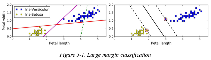
　　the solid line in the plot on the right represents the decision boundary of an SVM classifier；this line not only separates the two classes but also stays as far away from the closest training instances as possible.  you can think of an SVM classifier as fitting the widest possible street(represented by the parallel dashed lines) between the classes. this is called large margin classification. 

　　adding more training instances “off the street” will not affect the decision boundary at all: it is fully determined by the instances located on the edge of the street. these instances are called the support vectors. (they are circled in Figure5-1)

　　warning: SVMs are sensitive to the features scales，as you can see in Figure5-2: on the left plot，the vertical scale is much larger than the horizontal scale，so the widest possible street is close to horizontal. after feature scaling，the decision boundary looks much better(on the right polt). 

　　

Soft Margin Classification: 

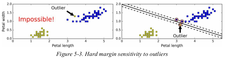
　　if we strictly impose that all instances be off the street and on the right side(严格要求所有实例都不在街上且都在正确的一边)，this is called hard margin classification. there are two main issues with hard margin classification. first，it only works if the data is linearly separable，and second it is quite sensitive to outliers. Figure 5-3 shows the iris dataset with just one additional outlier: on the left，it is impossible to find a hard margin，and on the right the decision boundary ends up very different from the one we saw in Figure 5-1 without the outlier，and it will probably not generalize as well. 

　　

　　to avoid these issues it is preferable to use a more flexible model. the objective is to find a good balance between keeping the street as large as possible and limiting the margin violations(i.e., instances that end up in the middle of the street or even on the wrong side). this is called soft margin classification. 

　　in Scikit-Learn's SVM classes，you can control this balance using the C hyperparameter: a smaller C value leads to a wider street but more margin violations. 

　　

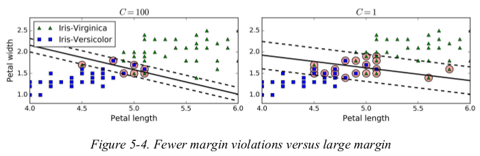
　　Figure 5-4 shows the decision boundaries and margins of two soft margin SVM classifiers on a nonlinearly separable dataset. on the left，using a high C value the classifier makes fewer margin violations but ends up with a smaller margin. on the right，using a low C value the margin is much larger，but many instances end up on the street. however，it seems likely that the second classifier will generalize better: in fact even on this training set it makes fewer prediction errors，since most of the margin violations are actually on the correct side of the decision boundary. 

　　if your SVM model is overfitting，you can try regularizing it by reducing C. 

from sklearn.svm import LinearSVC

iris = datasets.load_iris()
X = iris['data'][:, (2, 3)]
y = (iris['target'] == 2).astype(np.float64)

svm_clf = Pipeline([
    ('scaler', StandardScaler()),
    ('linear_svc', LinearSVC(C=1, loss='hinge')),
])
svm_clf.fit(X, y)

print(svm_clf.predict([[5.5, 1.7]]))  # [1.]

　　unlike Logistic Regression classifiers，SVM classifiers don't output probabilities for each class. 

　　alternatively，you could use the SGDClassifier class，with SGDClassifier(loss="hinge", alpha=1/(m*C)). this applies regular Stochastic Gradient Descent to train a linear SVM classifier. it doesn't converge as fast as the LinearSVC class，but it can be useful to handle huge datasets that don't fit in memory，or to handle online classification tasks. 

　　the LinearSVC class regularizes the bias term，so you should center the training set first by subtracting its mean. this is automatic if you scale the data using the StandardScaler. 

moreover，make sure you set the loss hyperparameter to “hinge”，as it not the default value. finally，for better performance you should set the dual hyperparameter to False，unless there are more features than training instances. 不让设置dual=False？？

Nonlinear SVM Classification: 

　　Polynomial Kernel

　　Adding Similarity Features

　　Guassian RBF Kernel

　　Computational Complexity

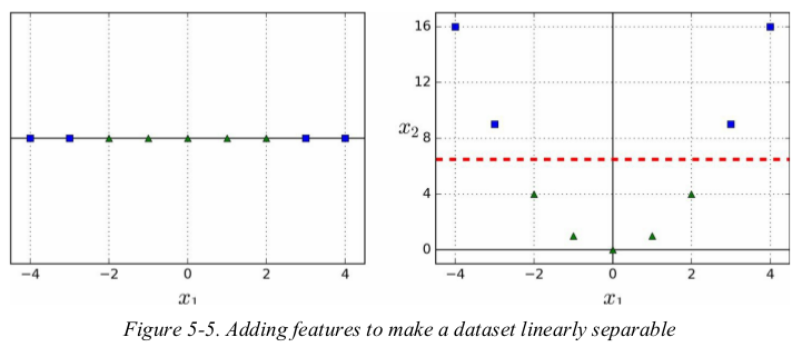
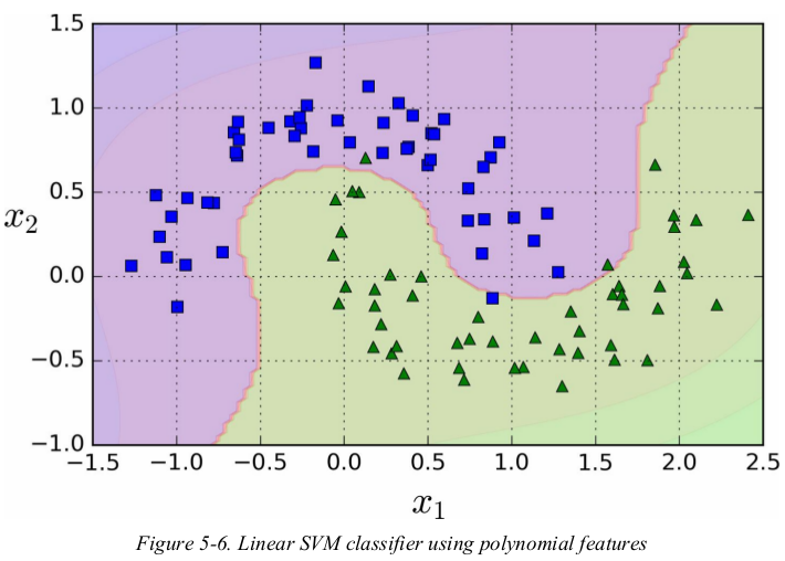
　　one approach to handling nonlinear datasets is to add more features，such as polynomial features；in some cases this can result in a linearly separable dataset. consider the left plot in Figure 5-5: it represents a simple dataset with just one feature x₁.  this dataset is not linearly separable，but if you add a second feature x₂ = (x₁)²，the resulting 2D dataset is perfectly linear separable. 

　　

　　示例: 

from sklearn.pipeline import Pipeline
from sklearn.preprocessing import PolynomialFeatures, StandardScaler
from sklearn.svm import LinearSVC

X, y = datasets.make_moons(n_samples=100, noise=0.15, random_state=42)

polynomial_svm_clf = Pipeline([
    ('poly_features', PolynomialFeatures(degree=3)),
    ('scaler', StandardScaler()),
    ('svm_clf', LinearSVC(loss='hinge', C=10, random_state=42))
])
polynomial_svm_clf.fit(X, y)


def plot_dataset(X, y, axes):
    plt.plot(X[:, 0][y == 0], X[:, 1][y == 0], "bs")
    plt.plot(X[:, 0][y == 1], X[:, 1][y == 1], "g^")
    plt.axis(axes)
    plt.grid(True, which='both')
    plt.xlabel(r"$x_1$", fontsize=20)
    plt.ylabel(r"$x_2$", fontsize=20, rotation=0)


def plot_predictions(clf, axes):
    x0s = np.linspace(axes[0], axes[1], 100)
    x1s = np.linspace(axes[2], axes[3], 100)
    x0, x1 = np.meshgrid(x0s, x1s)
    X = np.c_[x0.ravel(), x1.ravel()]
    y_pred = clf.predict(X).reshape(x0.shape)
    y_decision = clf.decision_function(X).reshape(x0.shape)
    plt.contourf(x0, x1, y_pred, cmap=plt.cm.brg, alpha=0.2)
    plt.contourf(x0, x1, y_decision, cmap=plt.cm.brg, alpha=0.1)


plot_predictions(polynomial_svm_clf, [-1.5, 2.5, -1, 1.5])
plot_dataset(X, y, [-1.5, 2.5, -1, 1.5])
plt.show()

　　

polynomial kernel: 

　　adding polynomial features is simple to implement and can work great with all sorts of Machine Learning algorithms (not just SVMs)，but at a low polynomial degree it can't deal with very complex datasets，and with a high polynomial degree it creates a huge number of features，making the model too slow. 

　　fortunately，when using SVMs you can apply an almost miraculous mathematical technique called the kernel trick. it makes it possible to get the same result as if you added many polynomial features，even with very high-degree polynomial，without actually having to add them. so there is no combinatorial explosion of the number of features since you don't actually add any features. this trick is implemented by the SVC class. 

from sklearn.pipeline import Pipeline
from sklearn.svm import SVC

X, y = datasets.make_moons(n_samples=100, noise=0.15, random_state=42)

poly_kernel_svm_clf = Pipeline([
    ('scaler', StandardScaler()),
    ('svm_clf', SVC(kernel='poly', degree=3, coef0=1, C=5)),
])
poly_kernel_svm_clf.fit(X, y)

　　the hyperparameter coef0 controls how much the model is influenced by high-degree polynomials versus low-degree polynomials. 

Adding Similarity Features: 

　　another technique to tackle nonlinear problems is to add features computed using a similarity function that measures how much each instance resembles a particular landmark.

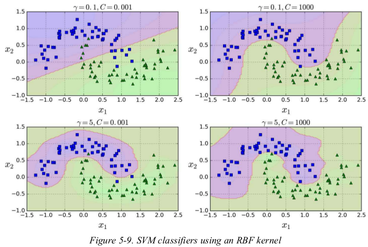
　　for example，let's take the one-dimensional dataset and add two landmarks to it at x₁ = -2 and x₁ = 1. next，let's define the similarity function to be the Gaussian Radial Basis Function (RBF) with γ =  0.3.(see Equation 5-1) 

　　

　　it is a bell-shaped function varying from 0 to 1. now we are ready to compute the new features. for example，let's look at the instance x₁ = -1: it is located at a distance of 1 from the first landmark，and 2 from the second landmark. therefore its new features are  the plot on the right of Figure 5-8 shows the transformed dataset. it is now linearly separable. 

　　

　　you may wonder how to select the landmarks. the simplest approach is to create a landmark at the location of each and every instance in the dataset. this creates many dimensions and thus increases the chances that the transformed training set will be linearly separable. 

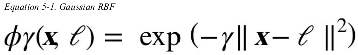
Gaussian RBF Kernel: 

　　just like the polynomial features method，the similarity features method can be useful with any Machine Learning algorithm，but it may be computationally expensive to compute all the additional features，especially on large training sets. however，once again the kernel trick does its SVM magic: 

from sklearn.svm import SVC

X, y = datasets.make_moons(n_samples=100, noise=0.15, random_state=42)

rbf_kernel_svm_clf = Pipeline([
    ('scaler', StandardScaler()),
    ('svm_clf', SVC(kernel='rbf', gamma=5, C=0.001)),
])
rbf_kernel_svm_clf.fit(X, y)

　　

　　increasing gamma makes the bell-shape curve narrower，the decision boundary ends up being more irregular，wiggling around individual instances. conversely，a small gamma value makes the bell-shaped curve wider，so instances have a larger range of influence，and the decision boundary ends up smoother. so gamma acts like a regularization hyperparameter: if your model is overfitting，you should reduce it，and if it is underfitting，you should increase it (similar to the C hyperparameter). 

　　

　　with so many kernels to choose from，how can you decide which one to use？as a rule of thumb，you should always try the linear kernel first (remember that LinearSVC is much faster than SVC(kernel=“linear”))，especially if the training set is very large or if it has plenty of features. if the training set is not too large，you should try the Gaussian RBF kernel as well；it works well in most cases. then if you have spare time and computing power，you can also experiment with a few other kernels using cross-validation and grid search，especially if there are kernels specialized for your training set's data structure. 

Computational Complexity: 

　　the LinearSVC class is based on the liblinear library，which implements an optimized algorithm for linear SVMs. it doesn't support the kernel trick，but it scales almost linearly with the number of training instances and the number of features: its training time complexity is roughly O(m × n).  

　　the algorithm takes longer if you require a very high precision. this is controlled by the tolerance hyperparameter (called tol in Scikit-Learn). in most classification tasks，the default tolerance is fine. 

　　the SVC class is based on the libsvm library，which implements an algorithm that supports the kernel trick. the training time complexity is usually between O(m² × n) and O(m² × n). unfortunately，this means that it gets dreadfully slow when the number of training instances gets large. this algorithm is perfect for complex but small or medium training set. however，it scales well with the number of features，especially with sparse features. in this case，the algorithm scales roughly with the average number of nonzero features per instance. 

　　

SVM Regression

　　与分类任务的目标相反: instead of trying to fit the largest possible street between two classes while limiting margin violations，SVM Regression tries to fit as many instances as possible on the street while limiting margin violations(i.e., instances off the street).  the width of the street is controlled by a hyperparameter ε. 

from sklearn.svm import LinearSVR

X, y = datasets.make_moons(n_samples=100, noise=0.15, random_state=42)

svm_reg = LinearSVR(epsilon=1.5)
svm_reg.fit(X, y)

　　

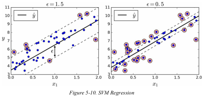
　　adding more training instances within the margin doesn't affect the model's predictions；thus，the model is said to be ε-insensitive. 

　　you can use Scikit-Learn's LinearSVR class to perform linear SVM Regression. 

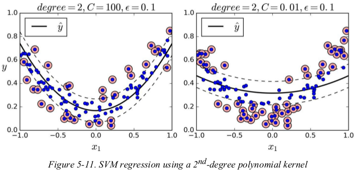
　　to tackle nonlinear regression tasks，you can use a kernelized SVM model. for example，Figure 5-11 shows SVM Regression on a random quadratic training set，using 2-degree polynomial kernel. there is little regularization on the left plot(i.e., a large C value)，and much more regularization on the right plot(i.e., a small C value). 

from sklearn.svm import SVR

X, y = datasets.make_moons(n_samples=100, noise=0.15, random_state=42)

svm_reg = SVR(kernel='poly', degree=2, C=100, epsilon=0.1)
svm_reg.fit(X, y)

　　

Under the Hood:  还没看？？

　　Decision Function and Predictions

　　Training Objective

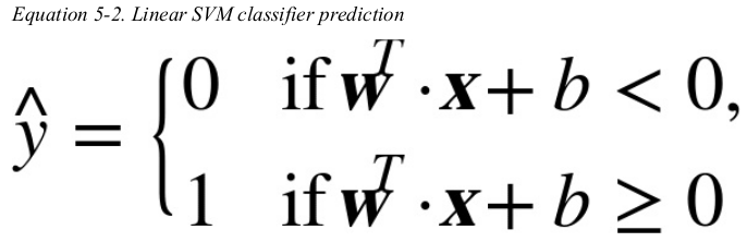
Decision Function and Predictions: 

　　the linear SVM classifier model predicts the class of a new instance x by simply computing the decision function: 

　　

Training Objective: 

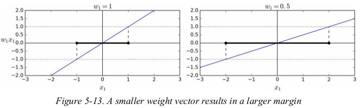
　　consider the slope of the decision function: it is equal to the norm of the weight vector，// w //. if we divide this slope by 2，the points where the decision function is equal to ±1 are going to be twice as far away from the decision boundary. in other words，dividing the slope by 2 will multiply the margin by 2. 还是没搞明白？？

　　

Exercises: 

1. What is the fundamental idea behind Support Vector Machines?

　　soft margin，

　　use kernels when training on nonlinear datasets.

2. What is a support vector?

　　including any instance located on the “street”

3. Why is it important to scale the inputs when using SVMs?

　　SVMs try to fit the largest possible “street” between the classes，so if the training set is not scaled，the SVMs will tend to neglect small features. 

4. Can an SVM classifier output a confidence score when it classifies an instance? What about a probability?

　　if you set probability=True when creating an SVM in Scikit-Learn，then after training it will calibrate the probabilities using Logistic Regression on the SVM's scores(trained by an additional five-fold cross-validation on the training data). this will add the predict_proba() and predict_log_proba() methods to the SVM. 

5. Should you use the primal or the dual form of the SVM problem to train a model on a training set with millions of instances and hundreds of features?

7. How should you set the QP parameters (H, f, A, and b) to solve the soft margin linear SVM classifier problem using an off-the-shelf QP solver?

8. Train a LinearSVC on a linearly separable dataset. Then train an SVC and a SGDClassifier on the same dataset. See if you can get them to produce roughly the same model.

from sklearn.svm import LinearSVC, SVC
from sklearn.linear_model import SGDClassifier

iris = datasets.load_iris()
X = iris["data"][:, (2, 3)]  # petal length, petal width
y = iris["target"]

setosa_or_versicolor = (y == 0) | (y == 1)
X = X[setosa_or_versicolor]
y = y[setosa_or_versicolor]

C = 5
alpha = 1 / (C * len(X))

lin_clf = LinearSVC(loss='hinge', C=C, random_state=42)
svm_clf = SVC(kernel='linear', C=C)
sgd_clf = SGDClassifier(loss='hinge', learning_rate='constant', eta0=0.001, alpha=alpha,
                        max_iter=100000, tol=-np.infty, random_state=42)

scaler = StandardScaler()
X_scaled = scaler.fit_transform(X)

lin_clf.fit(X_scaled, y)
svm_clf.fit(X_scaled, y)
sgd_clf.fit(X_scaled, y)

print(lin_clf.intercept_, lin_clf.coef_)
print(svm_clf.intercept_, lin_clf.coef_)
print(sgd_clf.intercept_, sgd_clf.coef_)
# [0.28474272] [[1.05364736 1.09903308]]
# [0.31896852] [[1.05364736 1.09903308]]
# [0.319] [[1.12072936 1.02666842]]

9. Train an SVM classifier on the MNIST dataset. Since SVM classifiers are binary classifiers, you will need to use one-versus-all to classify all 10 digits. You may want to tune the hyperparameters
using small validation sets to speed up the process. What accuracy can you reach?

from sklearn.svm import LinearSVC, SVC
from sklearn.metrics import accuracy_score

mnist = datasets.fetch_openml('mnist_784', version=1, cache=True)

X = mnist["data"]
y = mnist["target"]

X_train = X[:60000]
y_train = y[:60000]
X_test = X[60000:]
y_test = y[60000:]

np.random.seed(42)
rnd_idx = np.random.permutation(60000)
X_train = X_train[rnd_idx]
y_train = y_train[rnd_idx]

scaler = StandardScaler()
X_train_scaled = scaler.fit_transform(X_train)
X_test_scaled = scaler.transform(X_test)

# lin_clf = LinearSVC(random_state=42)
# lin_clf.fit(X_train, y_train)
# y_pred = lin_clf.predict(X_train)
# print(accuracy_score(y_train, y_pred))  #0.8946

# 仅标准化就能提高准确率
# lin_clf = LinearSVC(random_state=42)  # from scratch
# y_pred = lin_clf.fit(X_train_scaled, y_train)
# y_pred = lin_clf.predict(X_train_scaled)
# print(accuracy_score(y_train, y_pred))  # 0.9215166666666667

# 即使数据少了，准确率仍然提高了
# svm_clf = SVC(decision_function_shape='ovr', gamma='auto')  # OvR 或 OvO，创建多个二分类分类器
# svm_clf.fit(X_train_scaled[:10000], y_train[:10000])
# y_pred = svm_clf.predict(X_train_scaled)
# print(accuracy_score(y_train, y_pred))  # 0.9476

# 调参，使用很少的数据进行，之后再从头开始训练
from sklearn.model_selection import RandomizedSearchCV
from scipy.stats import reciprocal, uniform

svm_clf = SVC(decision_function_shape='ovr', gamma='auto')
param_distributions = {'gamma': reciprocal(0.001, 0.1), 'C': uniform(1, 10)}
rnd_search_cv = RandomizedSearchCV(svm_clf, param_distributions, n_iter=10, verbose=2, cv=3)
rnd_search_cv.fit(X_train_scaled[:1000], y_train[:1000])
print(rnd_search_cv.best_score_)  # 0.864
print(rnd_search_cv.best_params_)
rnd_search_cv.best_estimator_.fit(X_train_scaled, y_train)
y_pred = rnd_search_cv.best_estimator_.predict(X_train_scaled)
print(accuracy_score(y_train, y_pred))  # 0.99965
y_pred = rnd_search_cv.best_estimator_.predict(X_test_scaled)
print(accuracy_score(y_test, y_pred))  # 0.9728

10. Train an SVM regressor on the California housing dataset.

import numpy as np
from sklearn.datasets import fetch_california_housing
from sklearn.model_selection import train_test_split
from sklearn.preprocessing import StandardScaler
from sklearn.svm import LinearSVR
from sklearn.metrics import mean_squared_error
from sklearn.model_selection import RandomizedSearchCV

from sklearn.svm import SVR
from scipy.stats import reciprocal, uniform

housing = fetch_california_housing()
X = housing['data']
y = housing['target']

X_train, X_test, y_train, y_test = train_test_split(X, y, test_size=0.2, random_state=42)

scaler = StandardScaler()
X_train_scaled = scaler.fit_transform(X_train)
X_test_scaled = scaler.transform(X_test)

lin_svr = LinearSVR(random_state=42)
lin_svr.fit(X_train_scaled, y_train)

y_pred = lin_svr.predict(X_train_scaled)
mse = mean_squared_error(y_train, y_pred)
print(mse)  # 0.949968822217229
print(np.sqrt(mse))  # 0.9746634404845752


param_distributions = {'gamma': reciprocal(0.001, 0.1), 'C': uniform(1, 10)}
rnd_search_cv = RandomizedSearchCV(SVR(), param_distributions, n_iter=10, verbose=2, cv=3, random_state=42)
rnd_search_cv.fit(X_train_scaled, y_train)
y_pred = rnd_search_cv.best_estimator_.predict(X_train_scaled)
mse = mean_squared_error(y_train, y_pred)
print(np.sqrt(mse))  # 0.5727524770785356

y_pred = rnd_search_cv.best_estimator_.predict(X_test_scaled)
mse = mean_squared_error(y_test, y_pred)
print(np.sqrt(mse))  # 0.592916838552874

# capable of performing linear or nonlinear classification, regression, and even outlier detection.
# particularly well suited for classification of complex but small- or medium-sized datasets.

# Linear SVM Classification
# not only separates the these classes but also stays as far away from the closest training instances as possible. large margin classification.
#
# Notice that adding more training instances “off the street” will not affect the decision boundary at all:
# it is fully determined (or “supported”) by the instances located on the edge of the street. These instances are called the support vectors.
#
# SVMs are sensitive to the feature scales.

## Soft Margin Classification, 软间隔
# hard margin classification, strictly impose(严格规定) that all instances be off the street and on the right(正确的) side.
# There are two main issues with hard margin classification. First, it only works if the data is linearly separable, and second it is quite sensitive to outliers.
#
# soft margin classification, find a good balance between keeping the street as large as possible and limiting the margin violations (i.e.,
# instances that end up in the middle of the street or even on the wrong side).
# control this balance using the C hyperparameter: a smaller C value leads to a wider street but more margin violations.
# Figure5-4 shows the decision boundaries(决策边界) and margins of two soft margin SVM classifiers on a nonlinearly separable dataset.
# 右图 makes fewer prediction errors, since most of the margin violations are actually on the correct side of the decision boundary.

import numpy as np
from sklearn import datasets
from sklearn.pipeline import Pipeline
from sklearn.preprocessing import StandardScaler, PolynomialFeatures
from sklearn.svm import LinearSVC, SVC, LinearSVR, SVR

iris = datasets.load_iris()
X = iris['data'][:, (2, 3)]
y = (iris['target'] == 2).astype(np.float64)
# svm_clf = Pipeline([
#     ('std_scale', StandardScaler()),
#     ('linear_svc', LinearSVC(C=1, loss='hinge'))
# ])
# svm_clf.fit(X, y)
# print(svm_clf.predict([[5.5, 1.7]]))  # [1.]
# Unlike Logistic Regression classifiers, SVM classifiers do not output probabilities for each class.

# 也可以使用: SGDClassifier(loss="hinge", alpha=1/(m*C))
# It does not converge as fast as the LinearSVC class, but it can be useful to handle huge datasets that do not fit in memory (out-of-core training), or to handle online classification tasks.

# The LinearSVC class regularizes the bias term, so you should center the training set first by subtracting its mean. This is automatic if you scale the data using the StandardScaler.
# Moreover, make sure you set the loss hyperparameter to "hinge", as it is not the default value.
# Finally, for better performance you should set the `dual` hyperparameter to False, unless there are more features than training instances.


# Nonlinear SVM Classification
# 线性不可分变为线性可分: One approach to handling nonlinear datasets is to add more features, such as polynomial features; in some cases this can result in a linearly separable dataset.  # `this`指添加更多特征、
# polynomial_svm_clf = Pipeline([
#     ('poly_features', PolynomialFeatures(degree=3)),
#     ('std_scale', StandardScaler()),
#     ('linear_svc', LinearSVC(C=10, loss='hinge'))
# ])
# polynomial_svm_clf.fit(X, y)
# print(polynomial_svm_clf.predict([[5.5, 1.7]]))  # [1.]


## Polynomial Kernel
# at a low polynomial degree it cannot deal with very complex datasets, and with a high polynomial degree it creates a huge number of features, making the model too slow.
# kernel trick, It makes it possible to get the same result as if you added many polynomial features, even with very high-degree polynomials, without actually having to add them.
# The `coef0` controls how much the model is influenced by high-degree polynomials versus lowdegree polynomials.
# poly_kernel_svm_clf = Pipeline([
#     ('scaler', StandardScaler()),
#     ('svm_clf', SVC(kernel='poly', degree=3, coef0=1, C=5))
# ])
# poly_kernel_svm_clf.fit(X, y)


## Adding Similarity Features
# Another technique to tackle nonlinear problems is to add features computed using a similarity function that measures how much each instance resembles a particular landmark.
# 步骤, 1. take a dataset and add some landmarks to it
#       2. define the similarity function
#       3. compute the new features，有公式。之后数据线性可分。

# how to select the landmarks? The simplest approach is to create a landmark at the location of each and every instance in the dataset.
# This creates many dimensions and thus increases the chances that the transformed training set will be linearly separable.
# The downside is that a training set with m instances and n features gets transformed into a training set with m instances and m features (assuming you drop the original features).
# If your training set is very large, you end up with an equally large number of features.
# the kernel trick又用到了, it may be computationally expensive to compute all the additional features, especially on large training sets.


## Gaussian RBF Kernel
# rbf_kernel_svm_clf = Pipeline([
#     ('scaler', StandardScaler()),
#     ('svm_clf', SVC(kernel='rbf', gamma=5, C=0.001))
# ])
# rbf_kernel_svm_clf.fit(X, y)
# Increasing gamma makes the bell-shape curve narrower and as a result each instance’s range of influence is smaller:
# the decision boundary ends up being more irregular, wiggling around individual instances. So γ acts like a regularization hyperparameter:
# if your model is overfitting, you should reduce it, and if it is underfitting, you should increase it (similar to the C hyperparameter).  # 这里的C就是正则化参数。

# kernel的选择,
# 1. you should always try the linear kernel first.
# 2. If the training set is not too large, you should try the Gaussian RBF kernel as well; it works well in most cases.
# 3. Then if you have spare time and computing power, you can also experiment with a few other kernels using cross-validation and grid search, especially if there are kernels specialized for your training set’s data structure.

## Computational Complexity
# The LinearSVC class is based on the liblinear library, which implements an optimized algorithm for linear SVMs.
# It does not support the kernel trick, but it scales almost linearly with the number of training instances and the number of features: its training time complexity is roughly O(m × n).

# The SVC class is based on the libsvm library, which implements an algorithm that supports the kernel trick.
# The training time complexity is usually between O(m2 × n) and O(m3 × n). Unfortunately, this means that it gets dreadfully slow when the number of training instances gets large.
# This algorithm is perfect for complex but small or medium training sets.
# However, it scales well with the number of features, especially with sparse features (i.e., when each instance has few nonzero features). In this case, the algorithm scales roughly with the average number of nonzero features per instance.

# Table5-1. Comparison of Scikit-Learn classes for SVM classification


# SVM Regression
# instead of trying to fit the largest possible street between two classes while limiting margin violations,
# SVM Regression tries to fit as many instances as possible on the street  while limiting margin violations.

# The width of the street is controlled by a hyperparameter ϵ.  Figure5-10, ϵ是间隔线与决策边界在y轴方向上的长度。
# Adding more training instances within the margin does not affect the model’s predictions; thus, the model is said to be ϵ-insensitive.

# the training data should be scaled and centered first.
svm_reg = LinearSVR(epsilon=1.5)
svm_reg.fit(X, y)
# To tackle nonlinear regression tasks, you can use a kernelized SVM model.
# 正则化参数，大小变化与分类时一致

# The LinearSVR class scales linearly with the size of the training set (just like the LinearSVC class),
# while the SVR class gets much too slow when the training set grows large (just like the SVC class).
# supports the kernel trick.
svm_poly_reg = SVR(kernel='poly', degree=2, C=100, epsilon=0.1)
svm_poly_reg.fit(X, y)

# 支持核方法的是: SVC、SVR.

# 处理异常值，
# SVMs can also be used for outlier detection; see Scikit-Learn’s documentation for more details.


# Under the Hood
## Decision Function and Predictions
# Training a linear SVM classifier means finding the value of w and b that make this margin as wide as possible
# while avoiding margin violations (hard margin) or limiting them (soft margin).

## Training Objective
# the slope of the decision function is equal to the norm of the weight vector, ∥ w ∥. If we divide this slope by 2,
# the points where the decision function is equal to ±1 are going to be twice as far away from the decision boundary.
# So we want to minimize ∥ w ∥ to get a large margin.
#
# hard margin,
# Equation5-3, We are minimizing 1/2·wT · w, which is equal to 1/2·∥ w ∥2, rather than minimizing ∥ w ∥.
# This is because it will give the same result (since the values of w and b that minimize a value also minimize half of its square),
# but 1/2·∥ w ∥2 has a nice and simple derivative (it is just w) while ∥ w ∥ is not differentiable at w = 0.
# Optimization algorithms work much better on differentiable functions.
#
# soft margin,
# Equation5-4, ζ(i) measures how much the i^th instance is allowed to violate the margin.
# We now have two conflicting objectives: making the slack variables as small as possible to reduce the margin violations, and making 1/2·wT · w as small as possible to increase the margin.
# the tradeoff between these two objectives: C hyperparameter.

## Quadratic Programming, 二次规划
# The hard margin and soft margin problems are both convex quadratic optimization problems with linear constraints.
# Many off-the-shelf solvers are available to solve QP problems.

## The Dual Problem, 对偶问题
# Given a constrained optimization problem, known as the `primal problem`, it is possible to express a different but closely related problem, called its `dual problem`.
# The solution to the dual problem typically gives a lower bound to the solution of the primal problem, but under some conditions it can even have the same solutions as the primal problem.
# Luckily, the SVM problem happens to meet these conditions, so you can choose to solve the primal problem or the dual problem; both will have the same solution.

# The dual problem is faster to solve than the primal when the number of training instances is smaller than the number of features. More importantly,
# it makes the kernel trick possible, while the primal does not.

## Kernelized SVM, 核化支持向量机

## Online SVMs
# online learning means learning incrementally, typically as new instances arrive.

## hinge loss
# max(0, 1 – t). It is equal to 0 when t ≥ 1.
# Its derivative (slope) is equal to –1 if t < 1 and 0 if t > 1.
# It is not differentiable at t = 1, but just like for Lasso Regression you can still use Gradient Descent using any subderivative at t = 0 (i.e., any value between –1 and 0).