TF-IDF模型调参
1. 调TfidfVectorizer的参数 ngram_range, min_df, max_df:
上一篇博客调了ngram_range这个参数,得出了ngram_range=(1, 4)时效果最好这个结论,并在线上验证了下。
本篇博客继续调其他的参数。考虑到训练的速度,先将ngram_range设置为(1, 1),调min_df:
| min_df | train-mlogloss | val-mlogloss |
|---|---|---|
| 1 | 0.103793 | 0.406085 |
| 2 | 0.1091895 | 0.4051025 |
| 3 | 0.1098425 | 0.4057675 |
| 4 | 0.1105005 | 0.406762 |
通过以上调参可以看到,似乎min_df=2时在验证集上效果最好,再继续增大反而更差。
将ngram_range设置为(1, 2),可以看到:
| min_df | train-mlogloss | val-mlogloss |
|---|---|---|
| 1 | 0.0761615 | 0.3467905 |
| 2 | 0.071733 | 0.3457505 |
| 3 | 0.0752675 | 0.3465775 |
| 4 | 0.077503 | 0.3472625 |
ngram_range设置为(1, 2)时,也是min_df=2时效果最好。
调参数 max_df:
ngram_range设置为(1, 2),min_df设置为2。
| max_df | train-mlogloss | val-mlogloss |
|---|---|---|
| 1.0 | 0.071733 | 0.3457505 |
| 0.98 | 0.071733 | 0.3457505 |
| 0.95 | 0.071733 | 0.3457505 |
| 0.9 | 0.0827205 | 0.348275 |
| 0.8 | 0.083161 | 0.3503905 |
根据调参情况,max_df取1.0比较好。
比对线上结果:
在上一篇博客中,ngram_range=(1, 4), min_df=1, max_df=1.0得到的结果为:
train-mlogloss: 0.06831 val-mlogloss: 0.336836 test-mlogloss: 0.522686
现在只修改min_df=2,其他两个参数ngram_range=(1, 4), max_df=1.0:
train-mlogloss: 0.0696595 val-mlogloss: 0.336026 test-mlogloss: 0.524699
min_df调为2,在训练集和测试集上效果都不好了,仅在验证集上有些许提升,所以min_df的值应当取为1。
由此可见文件中的API,无论其数量多少,都是有用的。
最终TfidfVectorizer的参数设置为 ngram_range=(1, 4), min_df=1, max_df=1.0
2. 调xgboost的参数 subsample, colsample_bytree, max_depth, eta:
XGBoost参数解析:
eta [default=0.3, alias: learning_rate] 学习率
max_depth [default=6] 树的最大深度,可以用来防止过拟合,典型值是3-10
colsample_bytree [default=1] 列采样率,也就是特征采样率
subsample [default=1] 构建每棵树对样本的采样率,如果设置成0.5,XGBoost会随机选择一半的样本作为训练集
objective[默认reg:linear] 损失函数,multi:softprob:和softmax一样,但是返回的是每个数据属于各个类别的概率
num_class(softmax分类的个数)
eval_metric 对于有效数据的度量方法,mlogloss 多分类logloss损失函数
silent [default=0] 取0时表示打印出运行时信息,取1时表示以缄默方式运行,不打印运行时信息
# 上篇博客设置的参数:
param = {'max_depth': 6, 'eta': 0.1, 'eval_metric': 'mlogloss', 'silent': 1, 'objective': 'multi:softprob',
             'num_class': 8, 'subsample': 0.8, 'colsample_bytree': 0.85}
为了提高速度,先将ngram_range设置为(1, 2),TfidfVectorizer的其他参数不变。
subsample参数控制对于每棵树,随机采样的比例。 减小这个参数的值,算法会更加保守,避免过拟合。但是,如果这个值设置得过小,它可能会导致欠拟合。一般在0.5-1。
调参数subsample,xgboost的其他参数不变:
| subsample | train-mlogloss | val-mlogloss |
|---|---|---|
| 1.0 | 0.078896 | 0.348712 |
| 0.9 | 0.0770755 | 0.3458625 |
| 0.8 | 0.0761615 | 0.3467905 |
| 0.7 | 0.077435 | 0.3451595 |
| 0.6 | 0.0811085 | 0.3463795 |
| 0.5 | 0.0791555 | 0.348638 |
subsample可以取0.7-0.9之间的数。
3. 数据可视化:
训练集和测试集的数据分布:
上一篇博客中已计算出,训练集label统计:
import pandas as pd

train_path = './security_train.csv'
df = pd.read_csv(train_path)

df = df.drop(['api', 'tid', 'index'], axis=1)
df = df.drop_duplicates()

df['label'].value_counts() / df.label.count()
0 0.358465
5 0.308850
7 0.107079
2 0.086124
3 0.059048
6 0.037085
1 0.036149
4 0.007201
Name: label, dtype: float64
测试集label统计(通过线上提交数据获取):
提交文件中,将其中一列prob设为1,其他列置为0提交,共8次,得到一个test-mlogloss数组,
将其中一列设为0.3,其他列置为0.1提交,也是8次,再得到一个test-mlogloss数组。(代码中的result1, result2)
from math import log

result1 = [17.013720, 26.758693, 26.259607, 26.202020, 27.370820, 18.485384, 26.289467, 25.037486] # 全1全0
result2 = [2.772709, 3.248805, 3.224422, 3.221608, 3.278711, 2.844608, 3.225881, 3.164714] # 0.3 / 0.1

for i in range(0, len(result1)):
  result1[i] *= -12955

for i in range(0, len(result2)):
  result2[i] *= -12955

# 情况1:全1全0
# 预测正确 8*log(1-1e-6)
# 预测错误 6*log(1-1e-6) + 2*log(1e-6)

r = 8*log(1-1e-6)
e = 6*log(1-1e-6) + 2*log(1e-6)

# 情况2:0.3/0.1
# 预测0.3 log(0.3) + 7*log(0.9)
# 预测0.1 log(0.7) + log(0.1) + 6*log(0.9)
r2 = log(0.3) + 7*log(0.9)
e2 = log(0.7) + log(0.1) + 6*log(0.9)

lst = []
for i in range(0, len(result1)):
  temp = (result1[i] - 12955*e)/(r - e)
  lst.append(round(temp))
print(lst)

lst2 = []
for i in range(0, len(result2)):
  temp = (result2[i] - 12955*e2)/(r2 - e2)
  lst2.append(round(temp))
print(lst2 == lst)
[4978, 409, 643, 670, 122, 4288, 629, 1216]
True
import matplotlib.pyplot as plt
import numpy as np

trainlst = [4978, 502, 1196, 820, 100, 4289, 515, 1487]
testlst = [4978, 409, 643, 670, 122, 4288, 629, 1216]

for i in range(len(trainlst)):
  testlst[i] /= 12955
  trainlst[i] /= 13877

print("训练数据比例:", trainlst)
print("测试数据比例:", testlst)

# 绘制对比柱状图
bar_width = 0.3
plt.bar(x=range(len(trainlst)), height=trainlst, label="train data", alpha=0.8, width=bar_width)
plt.bar(x=np.arange(len(trainlst)) + bar_width, height=testlst, label="test data", alpha=0.8, width=bar_width)
plt.legend()
plt.xlabel("label")
plt.ylabel("percent")
plt.title('data distribution')
plt.show()
训练数据比例: [0.3587230669453052, 0.036174965770699716, 0.08618577502342005, 0.05909058153779635, 0.007206168480219067, 0.3090725661165958, 0.037111767673128196, 0.10715572530085754]
测试数据比例: [0.38425318409880355, 0.03157082207641837, 0.049633346198379, 0.05171748359706677, 0.00941721343110768, 0.33099189502122733, 0.048552682362022384, 0.09386337321497491]
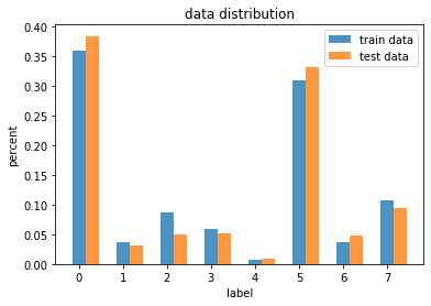
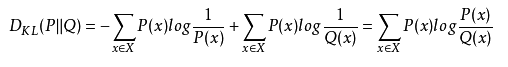
比较两个分布的差异:
KL散度:有时也称为相对熵,KL距离。对于两个概率分布P、Q,二者越相似,KL散度越小。KL散度是不对称的。
import numpy as np
import scipy.stats
p=np.asarray(trainlst)
q=np.asarray(testlst)
def KL_divergence(p,q):
    return scipy.stats.entropy(p, q)
print(KL_divergence(p,q))
print(KL_divergence(q,p))
0.016080060925276304
0.014372032451801856
测试集与训练集API数量分布的差异:
import pandas as pd

train_path = './security_train.csv'
df = pd.read_csv(train_path)

test_path = './security_test.csv'
df_test = pd.read_csv(test_path)

train_api_cnt = df.api.value_counts()
test_api_cnt = df_test.api.value_counts()

len(train_api_cnt) # 295
len(test_api_cnt) # 298

name_train = train_api_cnt.index.tolist()
value_train = train_api_cnt.tolist()
name_test = test_api_cnt.index.tolist()
value_test = test_api_cnt.tolist()

print("=== 只有训练集中有的api ===")
for i in range(len(train_api_cnt)):
  if name_train[i] not in name_test:
    print(name_train[i], value_train[i])

print("=== 只有测试集中有的api ===")
for i in range(len(test_api_cnt)):
  if name_test[i] not in name_train:
    print(name_test[i], value_test[i])
=== 只有训练集中有的api及调用次数 ===
RtlCompressBuffer 68
WSASendTo 2
EncryptMessage 1
=== 只有测试集中有的api及调用次数 ===
InternetGetConnectedStateExA 6
CreateDirectoryExW 4
MessageBoxTimeoutW 3
TaskDialog 1
NtDeleteFile 1
NtCreateUserProcess 1
由此可以看出,训练集和测试集调用的api有一些不同。
进一步分析训练集和测试集调用的api的数量差异:
name_differ = [] # 占比不同的api的名称
value_differ = [] # 加权过的api占比差值

rate = len(df) / len(df_test) # 权值 1.1326590184248322

for i in range(len(train_api_cnt)):
  if name_train[i] in name_test:
    differi = abs(value_train[i] - test_api_cnt[name_train[i]] * rate) / max(value_train[i], test_api_cnt[name_train[i]] * rate)
    if differi > 0.3:
      name_differ.append(name_train[i])
      value_differ.append(differi)

differ = pd.Series(value_differ, index=name_differ)
differ.sort_values(ascending=False)
recvfrom 0.987882
WSASend 0.977791
CryptEncrypt 0.969303
CertOpenSystemStoreA 0.954694
CryptUnprotectData 0.921522
...
CryptHashData 0.310428
CoCreateInstanceEx 0.306535
EnumServicesStatusW 0.306310
GetSystemDirectoryA 0.304643
GetFileVersionInfoW 0.302142
Length: 75, dtype: float64
简单通过数据集大小加权后,api调用的加权次数相比较,差值超过30%的api竟有75个之多。
由此可见虽然调用的api种类差不多,但数量上存在巨大差异。
虽然训练集和测试集的分布差异不大,但是api的调用次数比例差异很大。
由此可以得出一个初步结论:文件分类与api调用了多少次关系不大,可能与调用了哪种api以及api调用的序列有关。
以下从训练集来分析。
不同类别的文件调用api种类的差异:
不同label调用的api种类数:
df_temp = df.drop(['file_id', 'tid', 'index'], axis=1).drop_duplicates()
group_label = df_temp.groupby('label')
group_label['label'].count()
label
0 288
1 218
2 247
3 211
4 183
5 261
6 240
7 260
Name: label, dtype: int64
各种api出现在多少种文件中:
df_temp.groupby('api').label.count().sort_values(ascending=False)
api
NtOpenThread 8
NtQueryInformationFile 8
NtResumeThread 8
GetShortPathNameW 8
NtReadFile 8
..
InternetGetConnectedStateExW 1
CryptUnprotectData 1
GetUserNameExA 1
EncryptMessage 1
NetUserGetLocalGroups 1
Name: label, Length: 295, dtype: int64
简单统计了一下。
df_temp.groupby('api').label.count().sort_values(ascending=False).value_counts()
8 165
7 32
6 28
1 18
2 15
5 13
3 13
4 11
Name: label, dtype: int64
其中有一半以上的api是会出现在所有类型的文件中的,只出现在某一文件中的api很少。
由此可见,文件类型更多是与文件的行为有关,即api的调用序列有关,之后的模型训练应该主要从此下手。
组会总结
- 数据挖掘方向比较偏重于对于数据的统计特征之类的分析,组合特征做的比较好也可能带来很大的提升,文本处理方向侧重于用一些深度模型之类的方法来做;
- one-hot表示法的缺点:维度高,没法算距离;
- textcnn和n-gram比较相似,向前向后填充影响不会很大,但是lstm必须要在前面填充。(具体看paper)
- Xgboost调参
- Fasttest最新自动调参