【笔记】PyTorch框架学习 -- 2. 计算图、autograd以及逻辑回归的实现

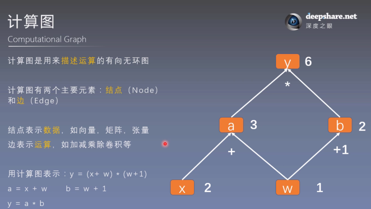
1. 计算图

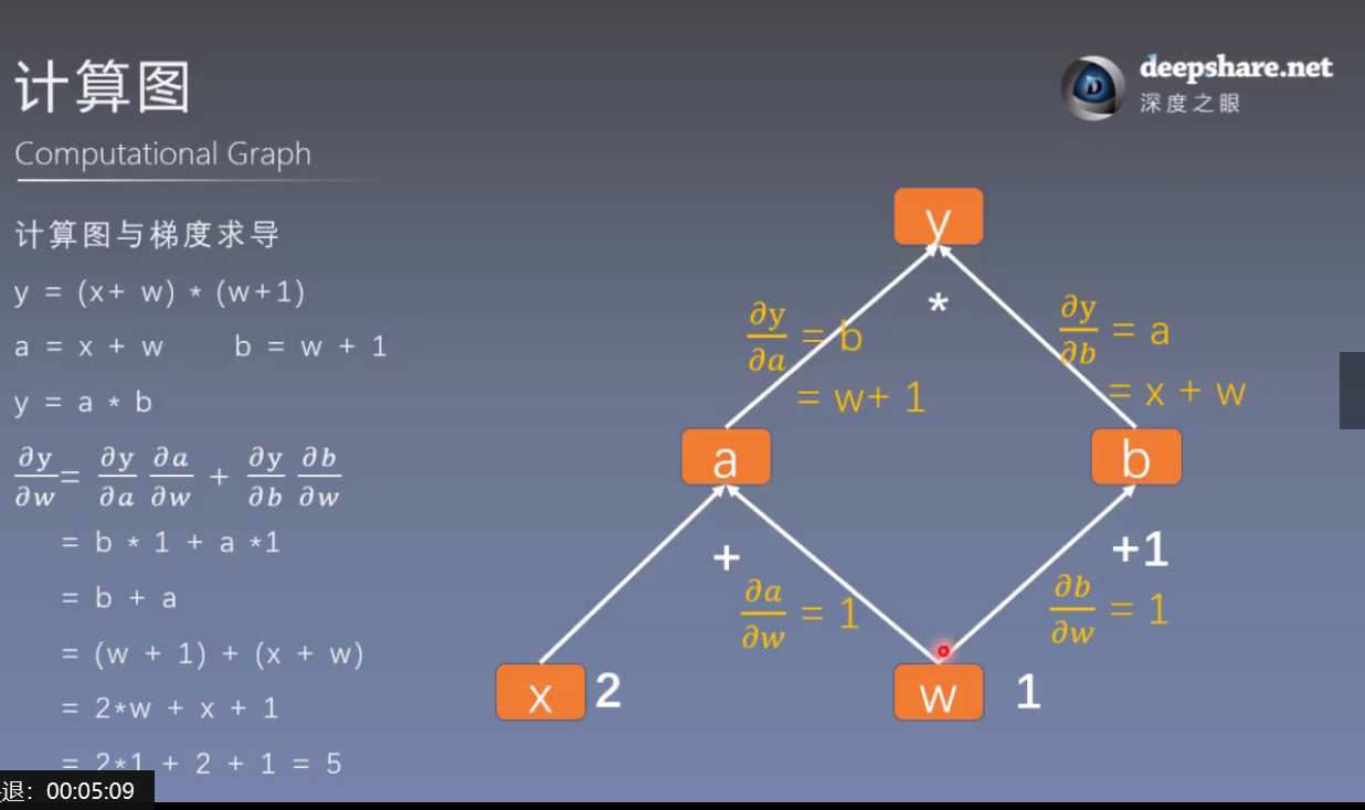
使用计算图的主要目的是使梯度求导更加方便。

import torch

w = torch.tensor([1.], requires_grad=True)
x = torch.tensor([2.], requires_grad=True)

a = torch.add(w, x)     # retain_grad()
b = torch.add(w, 1)
y = torch.mul(a, b)

y.backward()
print(w.grad) # tensor([5.])

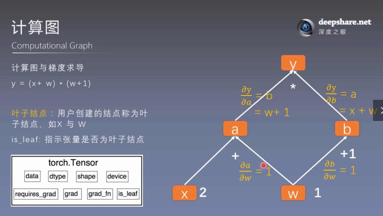
# 查看叶子结点
print("is_leaf:
", w.is_leaf, x.is_leaf, a.is_leaf, b.is_leaf, y.is_leaf)
# is_leaf: True True False False False

# 查看梯度
print("gradient:
", w.grad, x.grad, a.grad, b.grad, y.grad)
# gradient: tensor([5.]) tensor([2.]) None None None

# 查看 grad_fn
print("grad_fn:
", w.grad_fn, x.grad_fn, a.grad_fn, b.grad_fn, y.grad_fn)
# grad_fn:
# None 
# None 
# <AddBackward0 object at 0x00000258F55C28D0> 
# <AddBackward0 object at 0x00000258F55C2A58> 
# <MulBackward0 object at 0x00000258F55D5518>

2. 静态图和动态图

TensorFlow是静态图，PyTorch是动态图，区别在于在运算前是否先搭建图。

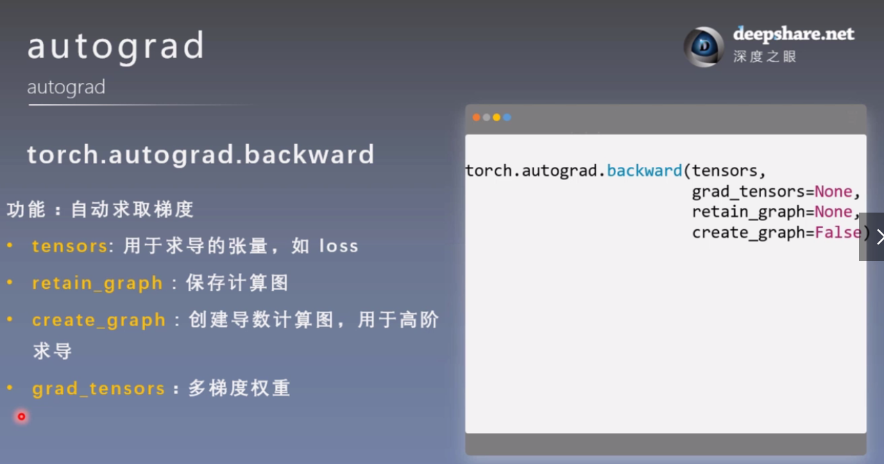
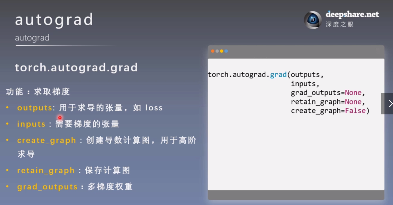
3. autograd 自动求导

import torch
torch.manual_seed(10)

# 非叶子节点默认不保存梯度，除非显式指定
w = torch.tensor([1.], requires_grad=True)
x = torch.tensor([2.], requires_grad=True)

a = torch.add(w, x)
b = torch.add(w, 1)
y = torch.mul(a, b)

# 如果不保存图，那么不能执行第二次
y.backward(retain_graph=True)
print(w.grad) # tensor([5.])
y.backward()

grad_tensors的使用：

w = torch.tensor([1.], requires_grad=True)
x = torch.tensor([2.], requires_grad=True)

a = torch.add(w, x)     # retain_grad()
b = torch.add(w, 1)

y0 = torch.mul(a, b)    # y0 = (x+w) * (w+1)
y1 = torch.add(a, b)    # y1 = (x+w) + (w+1)    dy1/dw = 2

loss = torch.cat([y0, y1], dim=0)       # [y0, y1]
print(loss) # tensor([6., 5.], grad_fn=<CatBackward>)

grad_tensors = torch.tensor([1., 2.])

loss.backward(gradient=grad_tensors)    # gradient 传入 torch.autograd.backward()中的grad_tensors

print(w.grad) # tensor([9.])

x = torch.tensor([3.], requires_grad=True)
y = torch.pow(x, 2)     # y = x**2

# 只有创建了导数的计算图，才能进行二阶求导
grad_1 = torch.autograd.grad(y, x, create_graph=True)   # grad_1 = dy/dx = 2x = 2 * 3 = 6
print(grad_1) # (tensor([6.], grad_fn=<MulBackward0>),)

grad_2 = torch.autograd.grad(grad_1[0], x)              # grad_2 = d(dy/dx)/dx = d(2x)/dx = 2，二阶导数
print(grad_2) # (tensor([2.]),)

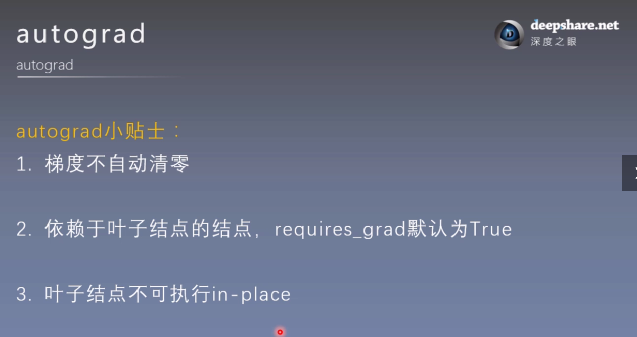
# 1. 梯度不自动清零
w = torch.tensor([1.], requires_grad=True)
x = torch.tensor([2.], requires_grad=True)

for i in range(4):
    a = torch.add(w, x)
    b = torch.add(w, 1)
    y = torch.mul(a, b)

    y.backward()
    print(w.grad)  # 若未清零，tensor([5.]) tensor([10.]) tensor([15.]) tensor([20.])

    w.grad.zero_() # 若清零了，tensor([5.]) tensor([5.]) tensor([5.]) tensor([5.])

# 2. 依赖叶子节点的节点，requires_grad默认为True
w = torch.tensor([1.], requires_grad=True)
x = torch.tensor([2.], requires_grad=True)

a = torch.add(w, x)
b = torch.add(w, 1)
y = torch.mul(a, b)

print(a.requires_grad, b.requires_grad, y.requires_grad) # True True True

# 查看下地址
a = torch.ones((1, ))
print(id(a), a) # 2158573461368 tensor([1.])

# a = a + torch.ones((1, ))
# print(id(a), a) # 1939675405912 tensor([2.]) 地址换了

a += torch.ones((1, ))
print(id(a), a) # 2158573461368 tensor([2.])

#===========================================

# 3. 叶子节点不能in-place操作
w = torch.tensor([1.], requires_grad=True)
x = torch.tensor([2.], requires_grad=True)

a = torch.add(w, x)
b = torch.add(w, 1)
y = torch.mul(a, b)

w.add_(1) # in-place操作，会报错

y.backward()

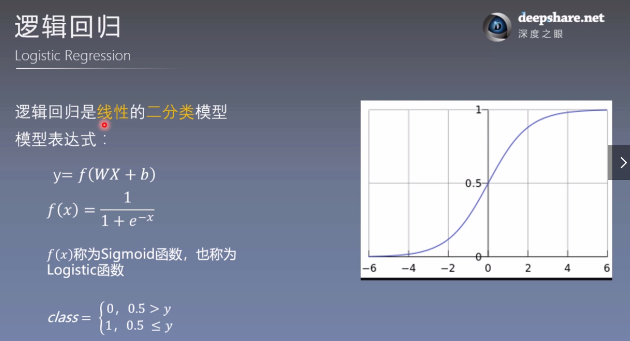
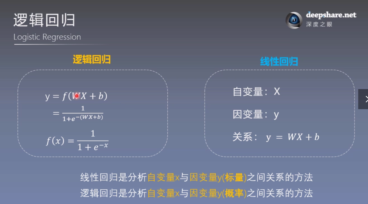
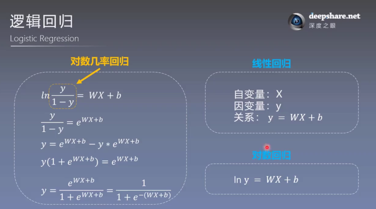
4. 逻辑回归

import torch
import torch.nn as nn
import matplotlib.pyplot as plt
import numpy as np
torch.manual_seed(10)


# ============================ step 1/5 生成数据 ============================
sample_nums = 100
mean_value = 1.7
bias = 1
n_data = torch.ones(sample_nums, 2)
x0 = torch.normal(mean_value * n_data, 1) + bias      # 类别0 数据 shape=(100, 2)
y0 = torch.zeros(sample_nums)                         # 类别0 标签 shape=(100, 1)
x1 = torch.normal(-mean_value * n_data, 1) + bias     # 类别1 数据 shape=(100, 2)
y1 = torch.ones(sample_nums)                          # 类别1 标签 shape=(100, 1)
train_x = torch.cat((x0, x1), 0)
train_y = torch.cat((y0, y1), 0)


# ============================ step 2/5 选择模型 ============================
class LR(nn.Module):
    def __init__(self):
        super(LR, self).__init__()
        self.features = nn.Linear(2, 1)
        self.sigmoid = nn.Sigmoid()

    def forward(self, x):
        x = self.features(x)
        x = self.sigmoid(x)
        return x


lr_net = LR()   # 实例化逻辑回归模型


# ============================ step 3/5 选择损失函数 ============================
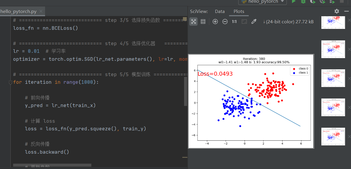
loss_fn = nn.BCELoss()

# ============================ step 4/5 选择优化器   ============================
lr = 0.01  # 学习率
optimizer = torch.optim.SGD(lr_net.parameters(), lr=lr, momentum=0.9)

# ============================ step 5/5 模型训练 ============================
for iteration in range(1000):

    # 前向传播
    y_pred = lr_net(train_x)

    # 计算 loss
    loss = loss_fn(y_pred.squeeze(), train_y)

    # 反向传播
    loss.backward()

    # 更新参数
    optimizer.step()

    # 清空梯度
    optimizer.zero_grad()

    # 绘图
    if iteration % 20 == 0:

        mask = y_pred.ge(0.5).float().squeeze()  # 以0.5为阈值进行分类
        correct = (mask == train_y).sum()  # 计算正确预测的样本个数
        acc = correct.item() / train_y.size(0)  # 计算分类准确率

        plt.scatter(x0.data.numpy()[:, 0], x0.data.numpy()[:, 1], c='r', label='class 0')
        plt.scatter(x1.data.numpy()[:, 0], x1.data.numpy()[:, 1], c='b', label='class 1')

        w0, w1 = lr_net.features.weight[0]
        w0, w1 = float(w0.item()), float(w1.item())
        plot_b = float(lr_net.features.bias[0].item())
        plot_x = np.arange(-6, 6, 0.1)
        plot_y = (-w0 * plot_x - plot_b) / w1

        plt.xlim(-5, 7)
        plt.ylim(-7, 7)
        plt.plot(plot_x, plot_y)

        plt.text(-5, 5, 'Loss=%.4f' % loss.data.numpy(), fontdict={'size': 20, 'color': 'red'})
        plt.title("Iteration: {}
w0:{:.2f} w1:{:.2f} b: {:.2f} accuracy:{:.2%}".format(iteration, w0, w1, plot_b, acc))
        plt.legend()

        plt.show()
        plt.pause(0.5)

        if acc > 0.99:
            break

最终结果：

思考：

1. 调整线性回归模型停止条件以及y = 2*x + (5 + torch.randn(20, 1))中的斜率，训练一个线性回归模型；
2. 计算图的两个主要概念是什么？
3. 动态图与静态图的区别是什么？
4. 逻辑回归模型为什么可以进行二分类？
5. 采用代码实现逻辑回归模型的训练，并尝试调整数据生成中的mean_value，将mean_value设置为更小的值，例如1，或者更大的值，例如5，会出现什么情况？
6. 再尝试仅调整bias，将bias调为更大或者负数，模型训练过程是怎么样的？