集成学习-梯度提升树

上篇博客已经讲了梯度提升树，但只讲了回归，本节讲一下分类，和一些进阶方法。

GBDT 分类

其实 GBDT 分类和回归思路基本相同，只是由于分类的标签是离散值，无法拟合误差，

解决办法有两种：一种是用指数损失函数，类似Adaboost，另一种是用类似于逻辑回归的对数似然损失函数，也就是输出类别预测的概率值，概率值连续，可以像回归一样拟合误差；

本文仅讨论 对数似然损失函数。

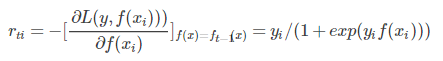
二分类

采用类似于逻辑回归的对数似然函数

y 取{-1,1}，是真实标签；此时的负梯度为　　

有了残差，就可以拟合出一棵 cart 树

　　　　　　　　　　　　

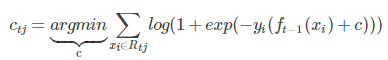
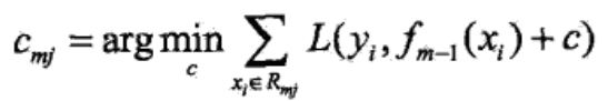
此时 cart 树已经能够建立了；

但是由于上式比较复杂，一般使用近似值替代

其余步骤都相同。

多分类

采用类似多分类的逻辑回归的对数似然函数

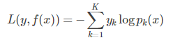
其实就是交叉熵，其中

即 softmax 。

知道这点就行，其他的有些复杂。

GBDT 正则化

注意，GBDT 并没有像 Adaboost 一样每步学习弱学习器，并没有对决策树有任何限制，可深可浅。

三种正则方法

1.  学习率，加法模型，都可以通过学习率防止过拟合

2. 子采样比例，只选取一部分样本来拟合 cart 树，注意比例不能太低

3. 对 cart 树剪枝

GBDT 实例

import numpy as np
import matplotlib.pyplot as plt

from sklearn import ensemble
from sklearn import datasets
from sklearn.utils import shuffle
from sklearn.metrics import mean_squared_error

# #############################################################################
# Load data
boston = datasets.load_boston()
print(boston.target)
X, y = shuffle(boston.data, boston.target, random_state=13)
X = X.astype(np.float32)
offset = int(X.shape[0] * 0.9)
X_train, y_train = X[:offset], y[:offset]
X_test, y_test = X[offset:], y[offset:]

# #############################################################################
# Fit regression model
params = {'n_estimators': 500, 'max_depth': 4, 'min_samples_split': 2,
          'learning_rate': 0.01, 'loss': 'ls'}
clf = ensemble.GradientBoostingRegressor(**params)

clf.fit(X_train, y_train)
mse = mean_squared_error(y_test, clf.predict(X_test))
print("MSE: %.4f" % mse)

# #############################################################################
# Plot training deviance

# compute test set deviance
test_score = np.zeros((params['n_estimators'],), dtype=np.float64)

for i, y_pred in enumerate(clf.staged_predict(X_test)):
    test_score[i] = clf.loss_(y_test, y_pred)

plt.figure(figsize=(12, 6))
plt.subplot(1, 2, 1)
plt.title('Deviance')
plt.plot(np.arange(params['n_estimators']) + 1, clf.train_score_, 'b-',
         label='Training Set Deviance')
plt.plot(np.arange(params['n_estimators']) + 1, test_score, 'r-',
         label='Test Set Deviance')
plt.legend(loc='upper right')
plt.xlabel('Boosting Iterations')
plt.ylabel('Deviance')

# #############################################################################
# Plot feature importance
feature_importance = clf.feature_importances_
# make importances relative to max importance
feature_importance = 100.0 * (feature_importance / feature_importance.max())
sorted_idx = np.argsort(feature_importance)
pos = np.arange(sorted_idx.shape[0]) + .5
plt.subplot(1, 2, 2)
plt.barh(pos, feature_importance[sorted_idx], align='center')
plt.yticks(pos, boston.feature_names[sorted_idx])
plt.xlabel('Relative Importance')
plt.title('Variable Importance')
plt.show()