
tidyr
> tdata <- data.frame(names=rownames(tdata),tdata)行名作为第一列
> gather(tdata,key="Key",value="Value",cyl:disp,mpg)创key列和value列,cyl和disp放在一列中
-号减去不需要转换的列
> spread(gdata,key="Key",value="Value")
根据value将key打散开 与unite函数对立
separate(df,col=x,into=c("A","B"))将数据框的列分割
unite(x,col="AB",A,B,sep='.')
dplyr
> dplyr::filter(iris,Sepal.Length>7)条件过滤
> dplyr::distinct(rbind(iris[1:10,],iris[1:15,]))去除重复行
> dplyr::slice(iris,10:15)切片
> dplyr::sample_n(iris,10)随机10行
> dplyr::sample_frac(iris,0.1)按比例随机选取
> dplyr::arrange(iris,Sepal.Length)排序
dplyr::arrange(iris,desc(Sepal.Length))降序
> select(starwars,height)选取
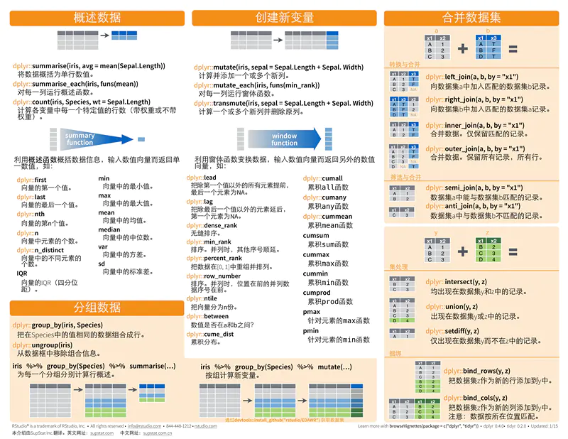
> summarise(iris,avg=mean(Sepal.Length))
统计函数
%>%链式操作符,管道 ctrl+shift+m
> iris %>% group_by(Species)
> dplyr::group_by(iris,Species)
> iris %>% group_by(Species) %>% summarise(avg=mean(Sepal.Width)) %>% arrange(avg)
> dplyr::mutate(iris,new= Sepal.Length+Petal.Length)相加总和
> dplyr::left_join(a,b,by="x1")
> dplyr::right_join(a,b,by="x1")
> dplyr::full_join(a,b,by="x1")
> dplyr::semi_join(a,b,by="x1")交集部分
> dplyr::anti_join(a,b,by="x1")补集部分
> intersect(first,second)交集
> dplyr::union_all(first,second)并集
> dplyr::union(first,second)非冗余并集
> setdiff(first,second)补集
heatmap输入矩阵
lm输入数据框
plot向量和向量-散点图,向量和因子-条形图
cbind,rbind矩阵或数据框
sum,mean,sd,range,median,sort,order向量
main 字符串不能为向量
na.rm true和false
axis side参数1到4
fig 包含四个元素向量
> plot(c(1:20),c(seq(1,89,length.out=20)),type="l",lty=1)实线
> plot(c(1:20),c(seq(1,89,length.out=20)),type="l",lty=2)虚线
数学统计
> x <- rnorm(n=100,mean=15,sd=2)生成100个平均数为15方差为2的随机数
> qqnorm(x)
set.seed(666) runif(50)绑定随机数
dgama(c(1:9),shape=2,rate=1)生成密度gama分布;随机数
描述性统计
summary()
fivenum()
Hmisc describe()
pastecs stat.desc() basic=T norm=T
psych describe() trim=0.1去除最低最高10%
> aggregate(Cars93[c("Min.Price","Price","Max.Price"," MPG.city")],by=list(Manufacturer=Cars93$Manufacturer),mean)字符串型 返回一个统计函数
doBy > summaryBy(mpg+hp+wt~am,data=myvars,FUN = mean)
psych describe.by(myvars,list(am=mtcars$am))分组统计
describeBy(myvars,list(am=mtcars$am))详细信息
统计函数 二元类元表
> table(cut(mtcars$mpg,c(seq(10,50,10))))频数统计
> prop.table(table(mtcars$cyl))频数占比
> table(Arthritis$Treatment,Arthritis$Improved)
> with(data=Arthritis,(table(Treatment,Improved)))省略数据集的名字
> xtabs(~Treatment+Improved,data=Arthritis)根据类别统计频数
> margin.table(x,1/2)总和
> addmargins(x)将总和添加到原表中
> ftable(y)评估式类元表
独立性检验
原假设:不变 备择假设:变化
P值越小越能实现
> mytable <- table(Arthritis$Treatment,Arthritis$Improved)
> chisq.test(mytable)卡方独立性检验
> fisher.test(mytable)精确独立检验
> mantelhaen.test(mytable)
> mytable <- xtabs(~Treatment+Sex+Improved,data=Arthritis)
> mantelhaen.test(mytable)
相关性检验
> cor(state.x77) > cor(x,y)
> cov(state.x77)
偏相关
ggm
> pcor(c(1,5,2,3,6),cov(state.x77))
> cor.test(state.x77[,3],state.x77[,5])
psych
> corr.test(state.x77)
> x <- pcor(c(1,5,2,3,6),cov(state.x77))
> pcor.test(x,3,50)
MASS
> t.test(Prob~So,data=UScrime)
绘图函数
散点图 x、y
直方图 因子
热力图 数据矩阵
象限图 因子、向量
> plot(women$height~women$weight)关联图
> fit <- lm(height~weight,data=women)
> plot(fit)
S3 par/plot/summary
> plot(as.factor(mtcars$cyl),col=c("red","yellow","blue"))
偏度是统计数据分布偏斜方向程度的度量,统计数据分布非对称程度数字特征、峰度是表征概率密度分布曲线在平均值处峰值高低的特征数
> mystats <- function(x,na.omit=FALSE){
+ if(na.omit)
+ x <- x[!is.na(x)]
+ m <- mean(x)
+ n <- length(x)
+ s <- sd(x)
+ skew <- sum((x-m^3/s^3))/n
+ kurt <- sum((x-m^4/s^4))/n-3
+ return(c(n=m,mean=m,stdev=s,skew=skew,kurtosis=kurt))
+ }
> i=1;while (i<=10){print("Hello,World");i=i+2;}
for(i in 1:10){print("Hello,World")}
> ifelse(score>60,print("PASS"),print("FAIL")
线性回归
> fit <- lm(weight~height,data=women)
> summary(fit)
> coefficients(fit)
> confint(fit,level=)置信区间,默认95%
> fitted(fit)拟合模型预测值
源数据-预测值=残差residuals()
> predict(fit,women1)根据结果对新数据进行预测
残差拟合图,正态分布图,大小位列图,残差影响图
plot(women$height,women$weight)
abline拟合曲线
> fit2 <- lm(weight~height+I(height^2),data=women)增加二次项
> lines(women$height,fitted(fit2),col="red")
将点连成线,根据拟合曲线
Pr(>|t|)估计系数为0假设的概率,小于0.05
Residual standard error残差越小越好
Multiple R-squared拟合值越大越好,解释数据量
F-statistic模型是否显著,越小越好
AIC比较回归值拟合度结果
MASS
stepAIC逐步回归法
leaps
regsubsets全子集回归法
> par(mfrow=c(2,2)) plot四幅图显示在同个画面
抽样验证法
500个数据进行回归分析,predict对剩下500个预测,比较残差值
单因素方差分析
> library(multcomp)
> attach(cholesterol)
> table(trt)
> aggregate(response,by=list(trt),FUN=mean) 分组统计平均值查看效果最好因子
> fit <- aov(response~ trt,data=cholesterol) 方差分析
> summary(fit) 看统计结果,方差结果看F值 越大组间差异越显著、P值衡量F值越小越可靠
协方差
> attach(litter)
> aggregate(weight,by=list(dose),FUN=mean)
> fit <- aov(weight~gesttime+dose,data=litter)
> summary(fit)
双因素方差分析
> attach(ToothGrowth)
> xtabs(~supp+dose)统计频率
> aggregate(len,by=list(supp,dose),FUN=mean)剂量越小两者差别越明显
> ToothGrowth$dose <- factor(ToothGrowth$dose)
> fit <- aov(len ~ supp*dose,data=ToothGrowth)
> summary(fit)
HH
> interaction.plot(dose,supp,len,type="b",
col=c("red","blue"),pch=c(16,18),
main = "Interaction between Dose and Supplement Type")
多元方差分析
> library(MASS)
> attach(UScereal)
> shelf <- factor(shelf)
> aggregate(cbind(calories,fat,sugars),by=list(shelf),FUN=mean)
> summary.aov(fit)每组测量值不同,差异结果显著
功效分析
> pwr.f2.test(u=3,sig.level=0.05,power=0.9,f2=0.0769)假设显著性水平为0.05,在90%置信水平下至少需要184个样本
pwr.anova.test(k=2,f=0.25,sig.level=0.05,power=0.9) 2组效率为0.25显著性水平为0.05,功效水平为90,结果为86*2
> data(breslow.dat,package = "robust")
> summary(breslow.dat)
> attach(breslow.dat)
fit <- glm(sumY~Base + Trt +Age,data=breslow.dat,family=poisson(link="log")) 广义线性模型拟合泊松回归 响应变量
逻辑回归
> data(Affairs,package="AER")
> summary(Affairs)
> table(Affairs$affairs)
> prop.table(table(Affairs$affairs))
> prop.table(table(Affairs$gender))
> Affairs$ynaffair[Affairs$affairs>0] <- 1
> Affairs$ynaffair[Affairs$affairs==0] <- 0
> Affairs$ynaffair <- factor(Affairs$ynaffair,levels=c(0,1),labels=c("No","Yes"))
> table(Affairs$ynaffair)
> attach(Affairs )
> fit <- glm(ynaffair~gender+age+yearsmarried+children+religiousness+education+occupation+rating,data=Affairs,family=binomial())
> summary(fit)
> fit1 <- glm(ynaffair~age+yearsmarried+religiousness+rating,data=Affairs,family=binomial())
> summary(fit1)
> anova(fit,fit1,test="Chisq")
主成分分析
> library(psych)
> fa.parallel(USJudgeRatings,fa="pc",n.iter=100)直线与X符号生成值大于一和100次模拟的平行分析
CPU
> pc <- principal(USJudgeRatings,nfactors=1,rotate="none",scores=FALSE)/scores=T pc1包含成分整合,观测变量与主成分的相关系数,h2指成分公因子的方差,主成分对每个变量的方差解释度,u2指方差无法被主成分解释的比例,SSloadings特定主成分相关联的标准化后的方差值,proportion var每个主成分对相关值的解释程度
因子分析
> library(psych)
> options(digits=2)
> covariances <- ability.cov$cov
> correlations <- cov2cor(covariances)
> fa.parallel(correlations,fa="both",n.obs=112,n.iter=100)
> fa.varimax <- fa(correlations,nfactors=2,rotate="varimax",fm="pa")
> fa.promax <- fa(correlations,nfactors=2,rotate="promax",fm="pa")
factor.plot(fa.promax,labels=rownames(fa.promax$loadings))
fa.diagram(fa.varimax,simple=FALSE)
fa<-fa(correlations,nfactors=2,rotate="none",fm="pa",score=TRUE)
fa$weight
library(arules)
data(Groceries)
> fit <- apriori(Groceries,parameter=list(support=0.01,confidence=0.5))
> inspect(fit)