Python科学计算三维可视化【完结】

中国MOOC《Pyhton计算计算三维可视化》总结

课程url：here ，教师：黄天宇，嵩天

下文的图片和问题，答案都是从eclipse和上完课后总结的，转载请声明。

Python数据三维可视化

1Introduction

1.1可视化计算工具

1.1.1TVTK 科学计算三维可视化基础

Mayavi                三维网格面绘制，三维标量场和矢量场绘制

TraitsUI               交互式三维可视化

SciPy                    拟合，线性差值，统计，插值

数据过滤器

需要安装的软件：VTK, Mayavi, numpy, PyQt4, Traits, TraitsUI

1.2内容组织

流体数据的标量可视化、矢量可视化实例

三维扫描数据（模型/地形）

三维地球场景可视化实例

曲线UI交互控制可视化

2基础运用

2.1TVTK入门

科学计算可视化主要方法

• 二维标量数据场：颜色映射法，等值线法，立体图/层次分割法
• 三维标量数据场：面绘制法，体绘制法
• 矢量数据场：直接法，流线法

下载python开源库网站：https://www.lfd.uci.edu/~gohlke/pythonlibs/ 这里基本上集成了python需要用到的各个库的资源。

VTK库安装方法是将文件放在<C:WINDOWSsystem32>下面，这样系统可以自动检测到并安装，安装在使用如下操作，在开始菜单栏，输入cmd，用管理员身份启动cmd，输入pip install xxx(VTK版本号)，有时候安装不行是因为pip需要更新，或者VTK文件放的位置不对，只要根据系统提示正确操作就行。

2.2创建一个基本三维对象

tvtk.CubeSource()的使用代码为s = tvtk.CubeSource(traits)

tvtk中CubeSource()的调用方式：

s = tvtk.CubeSource(x_length=1.0,y_length=2.0,z_length=3.0)

• x_length:立方体在X轴的长度
• y_length:立方体在Y轴的长度
• z_length:立方体在Z轴的长度

以下是s的输出结果：

  Debug: Off

  Modified Time: 1903583

  Reference Count: 2

  Registered Events:

    Registered Observers:

      vtkObserver (000001813DFDB520)

        Event: 33

        EventName: ModifiedEvent

        Command: 000001813DBFDF80

        Priority: 0

        Tag: 1

  Executive: 000001813D838460

  ErrorCode: No error

  Information: 000001813D864210

  AbortExecute: Off

  Progress: 0

  Progress Text: (None)

  X Length: 1

  Y Length: 2

  Z Length: 3

  Center: (0, 0, 0)

  Output Points Precision: 0

• 可以用s.x_length/s.y_length/s.z_length获取长方体在三个方向上的长度。
• CubeSource对象的方法

方法	说明
Set/get_x_length()	设置/获取长方体对象在X轴方向的长度
Set/get_y_length()	设置/获取长方体对象在Y轴方向的长度
Set/get_z_length()	设置/获取长方体对象在Z轴方向的长度
Set/get_center()	设置/获取长方体对象所在坐标系的原点
Set/get_bounds()	设置/获取长方体对象的包围盒

TVTK库的基本三维对象

三维对象	说明
CubeSource	立方体三维对象数据源
ConeSource	圆锥三维对象数据源
CylinderSource	圆柱三维对象数据源
ArcSource	圆弧三维对象数据源
ArrowSource	箭头三维对象数据源

比如建立圆锥model，输入

from tvtk.api import tvtk

s = tvtk.ConeSource(height=3.0,radius=1.0,resolution=36)

可以用s.height/s.radius/s.resolution（分辨率）查到高度，半径和分辨率的数据，如果要详细指导所有数据，可以用print(s)命令。

vtkConeSource (000001813DE1E0E0)

  Debug: Off

  Modified Time: 1903620

  Reference Count: 2

  Registered Events:

    Registered Observers:

      vtkObserver (000001813DFDC000)

        Event: 33

        EventName: ModifiedEvent

        Command: 000001813DBFDD40

        Priority: 0

        Tag: 1

  Executive: 000001813D839090

  ErrorCode: No error

  Information: 000001813D864120

  AbortExecute: Off

  Progress: 0

  Progress Text: (None)

  Resolution: 36

  Height: 3

  Radius: 1

  Capping: On

  Center: (0, 0, 0)

  Direction: (1, 0, 0)

  Output Points Precision: 0

2.3显示一个基本三维对象

2.3.1如何利用tvtk绘制三维图形

tvtk使用管线（pipeline）绘制三维图形，其中一下函数

CubeSource(xxx)

PolyDataMapper(xxx)

Actor(xxx)

Renderer(xxx)

RenderWindow(xxx)

RenderWindowInteracotor(xxx)

协作完成管线任务

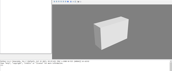
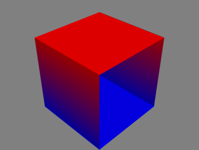
2.3.2实现一个三维长方体代码

代码例1

 from tvtk.api import tvtk

 s = tvtk.CubeSource(x_length=1.0,y_length=2.0,z_length=3.0)

 m = tvtk.PolyDataMapper(input_connection = s.output_port)

 a = tvtk.Actor(mapper=m)

 r = tvtk.Renderer(background=(0,0,0))

 r.add_actor(a)

 w = tvtk.RenderWindow(size=(300,300))

 w.add_renderer(r)

 i = tvtk.RenderWindowInteractor(render_window = w)

 i.initialize()

 i.start()

2.4TVTK管线与数据加载

• TVTK管线分两部分：数据预处理和图形可视化
• 数据预处理以s.output_port和m.input_connection形式输出
• 管线的两种类型：可视化管线（将原始数据加工成图形数据），图形管线（图形数据加工成图像）
• 可视化管线分两个对象：PolyData（计算输出一组长方形数据）和PolyDataMapper（通过映射器映射为图形数据）

TVTK对象	说明
Actor	场景中一个实体，描述实体位置，方向，大小的属性
Renderer	渲染作用，包括多个Actor
RenderWindow	渲染用的图形窗口，包括一个或多个Render
RenderWindowInteractor	交互功能，评议，旋转，放大缩小，不改变Actor或数据属性，只调整场景中照相机位置

• 管线的数据可以表示如下：

• 总结下TVTK管线就分为以下几个部分：数据预处理，数据映射，图形绘制，图形显示与交互
• 建立长方形模型：

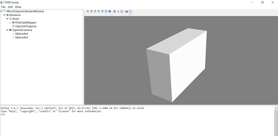
2.4.1IVTK观察管线

代码例2

 from tvtk.api import tvtk
 from tvtk.tools import ivtk
 from pyface.api import GUI
 s = tvtk.CubeSource(x_length=1.0,y_length=2.0,z_length=3.0)
 m = tvtk.Actor(mapper=m)
 gui = GUI()
 win = ivtk.IVTKWithCrustAndBrowser()
 win.open()
 True
 win.scene.add_actor(a)
 gui.start_event_loop()

显示结果：

有会出现bug，在主窗口缩放时左侧串口处于游离状态。

Debug程序：

 from tvtk.api import tvtk
 from tvtk.tools import ivtk
 from pyface.api import GUI
 s = tvtk.CubeSource(x_length=1.0,y_length=2.0,z_length=3.0)
 m = tvtk.PolyDataMapper(input_connection=s.output_port)
 a = tvtk.Actor(mapper=m)
 gui = GUI()
 win = ivtk.IVTKWithCrustAndBrowser()
 win.open()
 win.scene.add_actor(a)
 dialog = win.control.centralWidget().widget(0).widget(0)
 from pyface.qt import QtCore
 dialog.setWindowFlags(QtCore.Qt.WindowFlags(0x00000000))
 dialog.show()
 gui.start_event_loop()

Debug后第窗口界面，注意左侧的菜单栏，有分级

Model 建立后，可以在命令框输入代码，获取数据，比如：

输入print(scene.renderer.actors[0].mapper.input.points.to_array)，可以得到长方体各个顶点的坐标。

如果要集成开发，可以将函数单独封装，放到python.exe目录下，比如上一个生成长方体的代码可以封装成以下两部分：

主函数

from tvtk.api import tvtk
from tvtkfunc import ivtk_scene,event_loop
s = tvtk.CubeSource(x_length=1.0,y_length=2.0,z_length=3.0)
m = tvtk.PolyDataMapper(input_connection=s.output_port)
a = tvtk.Actor(mapper=m)
win = ivtk_scene(a)
win.scene.isometric_view()
event_loop()

调用函数

def ivtk_scene(actors):
    from tvtk.tools import ivtk
    # 创建一个带Crust（Python Shell）的窗口
    win = ivtk.IVTKWithCrustAndBrowser()
    win.open()
    win.scene.add_actor(actors)
    # 修正窗口错误
    dialog = win.control.centralWidget().widget(0).widget(0)
    from pyface.qt import QtCore
    dialog.setWindowFlags(QtCore.Qt.WindowFlags(0x00000000))
    dialog.show()
    return win

def event_loop():
    from pyface.api import GUI
    gui = GUI()
    gui.start_event_loop()

2.4.1Tvtk数据集（TVTK数据加载例1）

Tvtk中有5中数据集：

• ImageData表示二维/三维图像的数据结构，有三个参数，spacing,origin,dimensions

 from tvtk.api import tvtk
 img = tvtk.ImageData(spacing=(1,1,1),origin=(1,2,3),dimensions=(3,4,5))
 img.get_point(0)  #attain the data of first point
(1.0, 2.0, 3.0)
 for n in range(6):
...     print("%1.f,%1.f,%1.f"%img.get_point(n))

最后得到结果

1,2,3

2,2,3

3,2,3

1,3,3

2,3,3

3,3,3

• RectilinearGrid 表示创建间距不均匀的网格，所有点都在正交的网格上通过如下代码构建数据集：

 r.y_coordinates = y
 r.z_coordinates = z
 r.dimensions = len(x),len(y),len(z)
 r.x_coordinates = x
 r.y_coordinates = y
 r.z_coordinates = z
 r.dimensions = len(x),len(y),len(z)
 for n in range(6):
...     print(r.get_point(n))

得到数据结果，在轴上数据递增：

(0.0, 0.0, 0.0)

(3.0, 0.0, 0.0)

(9.0, 0.0, 0.0)

(15.0, 0.0, 0.0)

(0.0, 1.0, 0.0)

(3.0, 1.0, 0.0)

• StructuredGrid 表示创建任意形状网格，需要指定点的坐标
• PolyData 表示由一系列的点、点之间的联系以及由点构成的多边形组成
• UnstructuredGrid 无组织网格

TVTK数据集	特点
Imagedata	正交等间距
RectilinearGrid	正交不等间距
StructuredGrid	任意形状网格
PolyData	点和点之间的联系
UnstructuredGrid	无组织点

2.4.3Tvtk读取stl文件

STL文件调用形式：

S = tvtk.STLReader(file_name = “stl文件名”)

文件调用形式

vtkOBJReader()

ply文件调用形式

vtkPLYReader()

调用外部数据

VtkMultiBlockPLOT3DReander()

from tvtk.api import tvtk
from tvtkfunc import ivtk_scene,event_loop
s = tvtk.STLReader(file_name = 'python.stl')
m = tvtk.PolyDataMapper(input_connection = s.output_port)
a = tvtk.Actor(mapper=m)
win = ivtk_scene(a)
win.scene.isometric_view()
event_loop()

Stl格式数据，可以在python三维可视化中打开，也就是说solidworks中创建的stl文件也可以在python三维可视化中打开。

2.4.4Tvtk读取MultiBlock3D数据文件

3D文件读取用MultiBlock数据读取。

网格(XYZ文件)，空气动力学结果（Q文件），通用结果文件

源码：但是执行失败，错误类型是tvtk没有定义，或者plot3d没有定义

1.    from tvtk.api import tvtk
2.     
3.    def read_data():# 读入数据
4.        plot3d = tvtk.MultiBlockPLOT3DReader(
5.                xyz_file_name="combxyz.bin",#网格文件
6.                q_file_name="combq.bin",#空气动力学结果文件
7.                scalar_function_number=100,#设置标量数据数量
8.                vector_function_number=200#设置矢量数据数量
9.                )
10.        plot3d.update()
11.        return plot3d
12.     
13.    plot3d = read_data()
14.    grid = plot3d.output.get_block(0)

3VTK可视化基础实战

介绍三类可视化方法：标量可视化，矢量可视化，轮廓化可视化

3.1可视化实例

3.1.1标量可视化

等值面：标量值相等的面

Generate_value() 设定N条等值线的值，一般用于重新绘制等值线

Set_value() 设定一条等值线的值，一般用于覆盖某条等值线或者新增加一条等值线

代码例2：绘制流体数据模型的标量场

from tvtk.api import tvtk
from tvtkfunc import ivtk_scene,event_loop
plot3d = tvtk.MultiBlockPLOT3DReader(
...     xyz_file_name="combxyz.bin",
...     q_file_name="combq.bin",
...     scalar_function_number=100,vector_function_number=200)
plot3d.update()
grid=plot3d.output.get_block(0)
con = tvtk.ContourFilter()
con.set_input_data(grid)
con.generate_values(20,grid.point_data.scalars.range)
m = tvtk.PolyDataMapper(scalar_range=grid.point_data.scalars.range,input_connection=con.output_port)
a = tvtk.Actor(mapper=m)
a.property.opacity=0.5
win = ivtk_scene(a)    #以下3行为交互代码
win.scene.isometric_view()
event_loop()

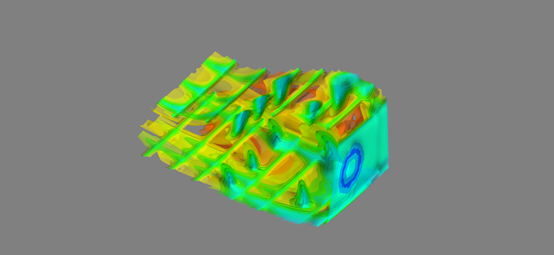
Generate_values(x,y)两个参数意义：x代表指定轮廓数，y代表数据范围

同样set_values(x,y)中也有同样的两个参数，含义相同，改变这两个参数会改变轮廓数和数据范围

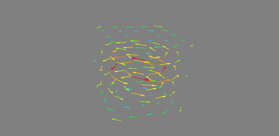
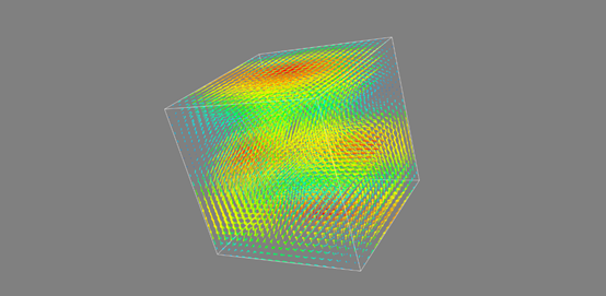
3.1.2矢量可视化

Tvtk.Glyph3D()               符号化技术，可以解决矢量数据可视化问题。

Tvtk.MaskPoints()          降采样

箭头表示标量大小，箭头方向表示矢量方向。

代码例3 矢量化向量

from tvtk.api import tvtk
from tvtkfunc import ivtk_scene,event_loop
plot3d = tvtk.MultiBlockPLOT3DReader(
...             xyz_file_name = "combxyz.bin",
...             q_file_name = "combq.bin",
...             scalar_function_number = 100,vector_function_number = 200)
plot3d.update()
grid = plot3d.output.get_block(0)
mask = tvtk.MaskPoints(random_mode=True,on_ratio=50)
mask.set_input_data(grid)
glyph_source = tvtk.ConeSource()
glyph = tvtk.Glyph3D(input_connection=mask.output_port,scale_factor=4)
glyph.set_source_connection(glyph_source.output_port)
m = vtk.PolyDataMapper(scalar_range=grid.point_data.scalars.range,input_connection=glyph.output_port)
a = tvtk.Actor(mapper = m)
win = ivtk_scene(a)
win.scene.isometric_view()
event_loop()

得到结果：

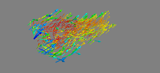
• vtk.Glyph3D()                          符号化技术

为了表示矢量数据，TVTK库中运用tvtk.Glyph3D()方法，同时运用MaskPoints()方法进行降维采样。

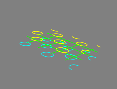
3.1.3空间轮廓线可视化

需要用到tvtk.StructuredGridOutlineFilter()

Python清空命令行代码函数：

Import os
def clear():
    os.system(‘cls’)
clear()

代码例4

from tvtk.api import tvtk
from tvtk.common import configure_input
from tvtkfunc import ivtk_scene, event_loop

plot3d = tvtk.MultiBlockPLOT3DReader(
        xyz_file_name="combxyz.bin",
        q_file_name="combq.bin",
        scalar_function_number=100, vector_function_number=200
    )#读入Plot3D数据
plot3d.update()#让plot3D计算其输出数据
grid = plot3d.output.get_block(0)#获取读入的数据集对象
outline = tvtk.StructuredGridOutlineFilter()#计算表示外边框的PolyData对象
configure_input(outline, grid)#调用tvtk.common.configure_input()
m = tvtk.PolyDataMapper(input_connection=outline.output_port)
a = tvtk.Actor(mapper=m)
a.property.color = 0.3, 0.3, 0.3
 
#窗口绘制
win = ivtk_scene(a)
win.scene.isometric_view()
event_loop()

显示结果

• PolyData对象的外边框处理使用了什么方法？

PolyData对象外边框使用了StructuredGridOutlineFilter()的方法。

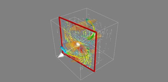
3.1.4结合矢量可视化和空间轮廓线可视化

对标量/轮廓属性进行赋值，不会处理。

from tvtk.api import tvtk
from tvtk.common import configure_input
from tvtkfunc import ivtk_scene, event_loop
plot3d = tvtk.MultiBlockPLOT3DReader(
...             xyz_file_name = "combxyz.bin",
...             q_file_name = "combq.bin",
...             scalar_function_number = 100,vector_function_number = 200)
plot3d.update()
grid = plot3d.output.get_block(0)
con = tvtk.ContourFilter()
con.set_input_data(grid)
con.generate_values(20,grid.point_data.scalars.range)  #20代表等值面
outline = tvtk.StructuredGridOutlineFilter()#计算表示外边框的PolyData对象
configure_input(outline, grid)#调用tvtk.common.configure_input()
m = tvtk.PolyDataMapper(scalar_range=grid.point_data.scalars.range,input_connection=con.output_port) 
m = tvtk.PolyDataMapper(input_connection=outline.output_port)
a = tvtk.Actor(mapper=m)
a.property.color = 0.3, 0.3, 0.3
a.property.opacity=0.5
win = ivtk_scene(a)    #以下3行为交互代码
win.scene.isometric_view()
event_loop()

3.2TVTK库实战练习

• 练习1：用tvtk绘制一个圆锥，圆锥的数据源对象为ConeSource(),圆锥高度为6.0,圆锥半径为2.0,背景色为红色。

代码例5

 from tvtk.api import tvtk
 from tvtk.tools import ivtk
 from pyface.api import GUI
 s = tvtk.ConeSource(height=6.0,radius=1.0,resolution=36)
 m = tvtk.PolyDataMapper(input_connection=s.output_port)
 a = tvtk.Actor(mapper=m)
 gui = GUI()
 win = ivtk.IVTKWithCrustAndBrowser()
 win.open()
 win.scene.add_actor(a)
 dialog=win.control.centralWidget().widget(0).widget(0)
 from pyface.qt import QtCore
 dialog.setWindowFlags(QtCore.Qt.WindowFlags(0x00000000))
 dialog.show()
 gui.start_event_loop()

代码例6

 from tvtk.api import tvtk
 s = tvtk.ConeSource(height=6.0,radius=2.0,resolution=36)
 m = tvtk.PolyDataMapper(input_connection=s.output_port)
 a = tvtk.Actor(mapper=m)
 r = tvtk.Renderer(background=(1,0,0))
 r.add_actor(a)
 w = tvtk.RenderWindow(size=(300,300))
 w.add_renderer(r)
 i = tvtk.RenderWindowInteractor(render_window=w)
 i.initialize()
 i.start()

• 练习2：使用tvtk库读取obj，并显示出来。

from tvtk.api import tvtk
from tvtkfunc import ivtk_scene,event_loop
s = tvtk.OBJReader(file_name = 'python.obj')
m = tvtk.PolyDataMapper(input_connection = s.output_port)
a = tvtk.Actor(mapper=m)
win = ivtk_scene(a)
win.scene.isometric_view()
event_loop()

• x.obj文件应该放在anaconda（python）安装目录下。
• Stl和obj模型包括哪些信息？

Stl全称是stereolithograph，模型包括三角面片数，每个三角面片的几何信息（法矢，三个顶点的坐标），三角面片属性。

Obj是3D模型文件模式，模型包括顶点数据，自由形态曲线/表面属性，元素，自由形态曲线/表面主题陈述，自由形态表面之间的连接，成组，显示/渲染属性。

• 练习3：通过get_value()和set_value()设定第一个等值面的值为原来的2倍

3.3Mayavi库入门

类别	说明
绘图函数	Barchar, contour3d, contour_surf, flow, imshow, mesh, plot3d, points3d, quiver3d, surf, triangular, mesh
图形控制函数	Clf, close, draw, figure, fcf, savefig, screenshot, sync_camera
图形修饰函数	Colorbar, scalarbar, xlabel, ylabel, zlabel
相机控制函数	Move, pitch, roll, view, set_engine
其他函数	Animate, axes, get_engine, show, set_engine
Mlat管线控制	Open, set_tvk_src,adddataset, scalar_cut_plane

Mayavi API

类别	说明
管线基础对象	Scene, source, filter, modulemanager, module, pipelinebase, engine
主视窗和UI对象	DecoratedScene, mayaviscene, sceneeditor, mlabscenemodel, engineview, enginerichview

3.3.1快速绘图实例

代码例7

#定义10个点的三维坐标,建立简单立方体

x = [[-1,1,1,-1,-1],[-1,1,1,-1,-1]]
y = [[-1,-1,-1,-1,-1],[1,1,1,1,1]]
z = [[1,1,-1,-1,1],[1,1,-1,-1,1]]
from mayavi import mlab
s = mlab.mesh(x,y,z)

代码例8

#建立复杂几何体

From numpy import pi,sin,cos,mgrid
from mayavi import mlab
dphi,dtheta = pi/250.0, pi/250.0
[phi,theta] = mgrid[0:pi+dphi*1.5:dphi,0:2*pi+dtheta*1.5:dtheta]
m0 = 4; m1 =3; m2 =2; m3 = 3; m4 = 6; m5= 2; m6 = 6; m7 = 4
r = sin(m0*phi)**m1 + cos(m2*phi)**m3 + sin(m4*theta)**m5 + cos(m6*theta)**m7
x = r*sin(phi)*cos(theta)
y = r*cos(phi)
z = r*sin(phi)*sin(theta)
s = mlab.mesh(x,y,z)
mlab.show()

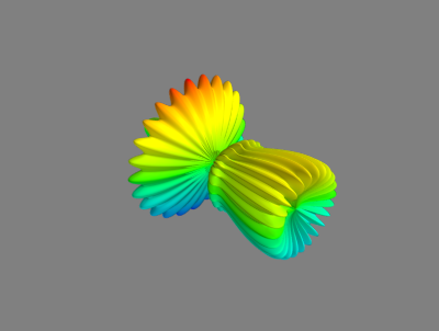
Mesh函数是三个二维的参数，点之间的连接关系，尤其由x,y,z之间的位置关系所决定。

上面这个例子如果改变代码行为mlab.mesh(x,y,z,representation="wireframe",line_width=1.0)

则结果为

3.3.2Mayavi管线（分析mayavi如何控制画面）

Mayavi管线的层级

• Engine：建立和销毁Scenes
• Scenes：多个数据集合Sources
• Filters：对数据进行变换
• Modules Manager：控制颜色，Colors and Legends
• Modules：最终数据的表示，如线条、平面等

程序配置属性的步骤：

• 获得场景对象，mlab.gcf()
• 通过children属性，在管线中找到需要修改的对象

配置窗口有多个选项卡，属性需要一级一级获得

s = mlab.gcf #获得s对象当前场景
print(s) #输出当前对象状态
print(s.scene.background) #输出当前设置的场景的背景色
source = s.children[0] #获取对象
print(repr(source)) #输出mlab儿子数组对象的第一个值地址
print(source.name) #返回该节点名称
print(repr(source.data.points)) #输出该节点坐标
print(repr(source.data.point_data.scalars))
manager = source.children[0] #数据源法向量
print(manager)
#通过程序更改物体颜色和对应颜色值
colors = manager.children[0]
colors.scalar_lut_manager.show_legend = True
surface = colors.children[0] #获取颜色的第一个子节点。Surface可以设置图形的显示方式
surface.actor.property.representation = “wireframe”
surface.actor.property.opacity = 0.6 #透明度设置为0.6

mayavi与tvtk处理三维可视化的异同点：tvtk处理三维可视化要通过映射，预处理步骤，而mayavi在获取数据，可以通过mlab.mesh(x,y,z)生成三维可视化图形。

3.4Mayavi库入门

3.4.1基于numpy数组的绘图函数

• Mlab对numpy建立可视化过程：

1. 建立数据源
2. 使用filter(可选)
3. 添加可视化模块

3D绘图函数-Points3d()

• 函数形式：

Points3d(x,y,z,…)            points3d(x,y,z,s,...)         points3d(x,y,z,f,…)

X,y,z便是numpy数组、列表或者其他形式的点三维坐标

s表示在该坐标点处的标量值

F表示通过函数f(x,y,z)返回的标量值

代码例9

t = np.linspace(0, 4 * np.pi, 20)
x = np.sin(2 * t)
y = np.cos(t)
z = np.cos(2 * t)
s = 2 + np.sin(t)
points = mlab.points3d(x,y,z,s,colormap='Reds',scale_factor=.25)

参数	说明
Color	VTK对象的颜色，定义为（0,1）的三元组
Colormap	Colormap的类型，例如Reds、Blues、Copper等
Extent	x,y,z数组范围[xmin,xmax,ymin,ymax,zmin,zmax]
Figure	画图
Line_width	线的宽度，该值为float，默认为0.2
Mask_points	减小/降低大规模点数据集的数量
Mode	符号的模式，例如2darrow、2dcircle、arrow、cone等
Name	VTK对象名字
Opcity	VTK对象的整体透明度，改值为float型，默认为1.0
Reset_zoom	对新加入场景数据的缩放进行重置。默认为True
Resolution	符号的分辨率，如球体的细分数，该值为整型，默认为8
Scale_factor	符号放缩的比例
Scale_mode	符号的放缩模式，如vector、scalar、none
Transparent	根据标量值确定actor的透明度
Vmax	对colormap放缩的最大值
Vmin	对colormap放缩的最小值

• 3D绘图函数-Plot3d()

函数形式：

Plot3d(x,y,z…)   plot3d(x,y,z,s,…)

X,y,z表示numpy数组，或列表。给出了线上连续的点的位置。S表示在该坐标点处的标量值

参数	说明
Tube_radius	线管的半径，用于描述线的粗细
Tube_sides	表示线的分段数，该值为整数，默认为6

X,y,z表示numpy数组，给出了线上连续的点的位置。

Np.sin(mu)表示在该坐标点处的标量值

Tube_radius绘制线的半径为0.025

Colormap采用Spectral颜色模式

代码例10

import numpy as np
from mayavi import mlab
n_mer, n_long = 6,11
dphi = np.pi / 1000.0
phi = np.arange(0.0, 2 * np.pi + 0.5 * dphi, dphi)
mu = phi * n_mer
x = np.cos(mu) * (1 + np.cos(n_long * mu / n_mer) * 0.5)
y = np.sin(mu) * (1 + np.cos(n_long * mu / n_mer) * 0.5)
z = np.sin(n_long * mu /n_mer) * 0.5
l = mlab.plot3d(x,y,z,np.sin(mu),tube_radius=0.025,colormap="Spectral")

X,y,z便是numpy数组，给出了线上连续的点的位置。

Np.sin(mu)表示在该坐标点处的标量值

Tube_radius绘制线的半径为0.025

Colormap采用Spectral颜色模式

• 3D绘图函数-2D数据

Imshow()-3D绘图函数

Interpolate        图像中的像素是否被插值，该值为布尔型，默认为True

代码例11

import numpy
from mayavi import mlab
s = numpy.random.random((10,10))
img = mlab.imshow(s,colormap='gist_earth')
mlb.show()

3D绘图函数 - surf()

函数形式：

Surf(s,...)
Surf(x,y,s…)
Surf(x,y,f,..)

S是一个高程矩阵，用二维数组表示

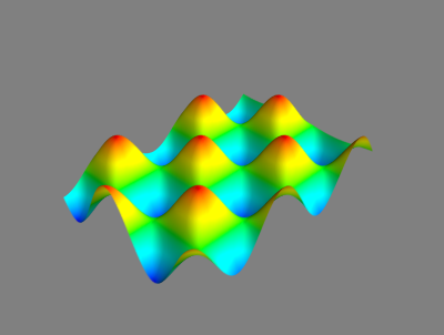
代码例12

import numpy as np
from mayavi improt mlab
from mayavi import mlab
def f(x,y):
    return np.sin(x - y) + np.cos(x + y)
x, y = np.mgrid[-7.:7.05:0.1,-5.:5.05:0.05]
s = mlab.surf(x,y,f)
mlab.show()

3D绘制函数 - contour_surf()，与surf()类似求解曲面，contour_surf求解等值线

代码例13

import numpy as np
from mayavi import mlab
def f(x,y):
    return np.sin(x - y) + np.cos(x + y)
x,y = np.mgrid[-7.:7.05:0.1,-5.:5.05:0.05]
con_s = mlab.contour_surf(x,y,f)

3D绘图函数 - contour3d()

函数形式：

Contour3D(scalars…)

Contour3d(x,y,z,scalar,..)

Scalars 网络上的数据，用三维numpy数组shuming，x,y,z代表三维空间坐标

参数	说明
Contours	定义等值面的数量

代码例14

import numpy
from mayavi import mlab
x,y,z = numpy.ogrid[-5:5:64j,-5:5:64j,-5:5:64j]
scalars = x * x + y * y + z * z
obj = mlab.contour3d(scalars, contours=8,transparent=True)

3D绘图函数 – quiver3d()

函数形式：

quiver3d(u,v,w…)

quiver3d(x,y,z,u,v,w…)

quiver3d(x,y,z,f,…)

u,v,w用numpy数组表示的向量

x,y,z表示箭头的位置，u,v,w矢量元素

f需要返回咋给定位置（x,y,z）的(u,v,w)矢量

代码例15

r = np.sqrt(x ** 2 + y ** 2 + z ** 4)
u = y * np.sin(r) / (r + 0.001)
v = -x * np.sin(r)/ (r + 0.001)
w = np.zeros_like(z)
obj = mlab.quiver3d(x,y,z,u,v,w,line_width=3,scale_factor=1)

Questions:

1. points3D和Plot3D两个函数之间的区别于联系是什么？
2. Imshow()方法是如何确定二维数组可视化图像颜色的？
3. Surf()方法实例中通过什么方法获取x,y二维数组的？
4. Mlab中可以进行矢量数据可视化的方法有哪些？

Corresponding answers:

1. Points3D是基于Numpy数组x,y,z提供的数据点坐标，绘制图形；Plot3D是基于1维numpy数组x,y,z供的三维坐标数据绘制图形；
2. Imshow()通过colormap关键字确定颜色，比如colormap='gist_earth'，确定颜色为“类似地球表面颜色”；
3. Surf()方法是通过np.mgrid(xxx,xxx)获取x,y二维数组；
4. mlab.Flow()和mlab.quiver3d()

3.4.2改变物体的外观

• 改变颜色

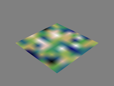
代码例16

Colormap定义的颜色，也叫LUT即look up table.

import numpy as np
from mayavi import mlab
x,y = np.mgrid[-10:10:200j,-10:10:200j]
z = 100 * np.sin(x * y) / (x * y)
mlab.figure(bgcolor=(1,1,1))
<mayavi.core.scene.Scene object at 0x00000214003D6678>
surf = mlab.surf(z,colormap='cool')
mlab.show()

代码例17

当代码例16增加以下代码到代码例17时，图像的颜色变淡，透明度增加。

import numpy as np
from mayavi import mlab
#建立数据
x,y = np.mgrid[-10:10:200j,-10:10:200j]
z = 100 * np.sin(x * y) / (x * y)
#对数据进行可视化
mlab.figure(bgcolor=(1,1,1))
<mayavi.core.scene.Scene object at 0x00000214003D6678>
surf = mlab.surf(z,colormap='cool')
mlab.show()
#访问surf对象的LUT
#LUT是一个255x4的数组，列向量表示RGBA，每个值的范围从0-255
lut = surf.module_manager.scalar_lut_manager.lut.table.to_array()
#增加透明度，修改alpha通道
lut[:,-1] = np.linspace(0,255,256)
surf.module_manager.scalar_lut_manager.lut.table = lut
#更新视图，并显示图像
mlab.show()

3.4.3Mlab控制函数

图像控制函数：

函数图像	说明
Clf	清空当前图像mlab.clf(figure=None)
close	关闭图形窗口 mlab.close(scene=None, all=False)
Draw	重新绘制当前图像mlab.close(figure=None)
Figure	建立一个新的scene或者访问一个存在的scene mlab.figure(figure=None,bgcolor=None,fgcolor=None,engine=None,size=(400,350))
Gcf	返回当前图像的handle mlab.gcf(figure=None)
Savefig	存储当前的前景，输出为一个文件，如png,jpg,bmp,tiff,pdf,obj,vrml等

图像装饰函数

函数图像	说明
Cololorbar	为对象的颜色映射增加颜色条
Scalarbar	为对象的标量颜色映射增加颜色条
Vectorbar	为对象的矢量颜色映射增加颜色条
xlabel	建立坐标轴，并添加x轴的标签mlab.xlabel(text,object=None)
Ylabel	建立坐标轴，并添加y轴的标签
zlabel	建立坐标轴，并添加z轴的标签

相机控制函数

函数图像	说明
Move	移动相机和焦点 Mlab.move(forward=None,right=None,up=None)
Pitch	沿着“向右”轴旋转角度mlab.pitch(degrees)
View	设置/获取当前视图中相机的视点 Mlab.view(azimuth=None,elevation=None,distance=None,focalpoint=None,roll=None Reset_roll=True,figure=None
Yaw	沿着“向上”轴旋转一定角度，mlab.yaw(degrees)

其他控制函数

函数图像	说明
animate	动画控制函数mlab.animate(func=None,delay=500,ui=True)
Axes	为当前物体设置坐标轴mlab.axes(*args,**kwargs)
Outline	为当前物体建立外轮廓mlab.outline(*args,**kwargs)
Show	与当前图像开始交互mlab.show(func=None,stop=False)
Show_pipeline	显示mayavi的管线对话框，可以进行场景属性的设置和编辑
Text	为图像添加文本mlab.text(*args,**kwargs)
Title	为绘制图像建立标题mlab.title(*args,**kwargs)

3.4.4鼠标选取交互操作

On_mouse_pick(callback,type=”point”,Button=”left”,Remove=False)提供鼠标响应操作

Type:”point”,”cell” or “world”

Button:”Left”,”Middle” or “Right”

Remove:如果值为True,则callback函数不起作用

返回：一个vtk picker对象

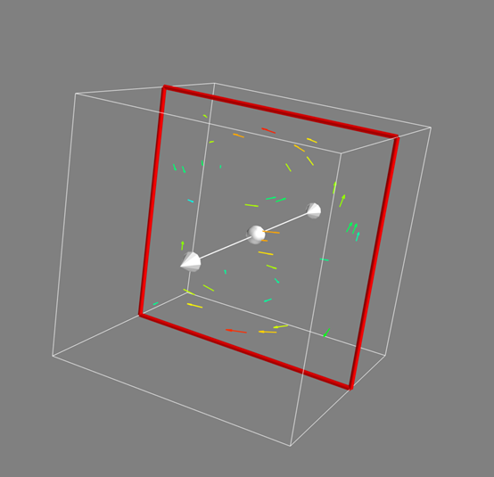
代码例18

程序框架：

#场景初始化
figure = mlab.gcf()
#用mlab.points3d建立红色和白色小球的集合
#
… …
#处理选取事件
def picker_callback(picker)
#建立响应机制
Picker = figure.on_mouse_pick(picker_callback)
mlab.show()
import numpy as np
from mayavi import mlab
figure = mlab.gcf()
x1, y1, z1 = np.random.random((3, 10))
red_glyphs = mlab.points3d(x1, y1, z1, color=(1, 0, 0),
                           resolution=10)
x2, y2, z2 = np.random.random((3, 10))
white_glyphs = mlab.points3d(x2, y2, z2, color=(0.9, 0.9, 0.9),
                             resolution=10)
outline = mlab.outline(line_width=3)
outline.outline_mode = 'cornered'
outline.bounds = (x1[0] - 0.1, x1[0] + 0.1,
                  y1[0] - 0.1, y1[0] + 0.1,
                  z1[0] - 0.1, z1[0] + 0.1)
glyph_points = red_glyphs.glyph.glyph_source.glyph_source.output.points.to_array()
def picker_callback(picker):
    if picker.actor in red_glyphs.actor.actors:
        point_id = int(picker.point_id / glyph_points.shape[0]) 
        if point_id != -1:
            x, y, z = x1[point_id], y1[point_id], z1[point_id]
            outline.bounds = (x - 0.1, x + 0.1,
                              y - 0.1, y + 0.1,
                              z - 0.1, z + 0.1)
picker = figure.on_mouse_pick(picker_callback)
mlab.title('Click on red balls')
mlab.show()

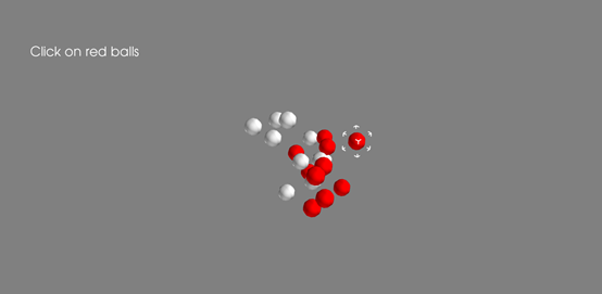
简述选取红色小球问题分析实例程序的基本框架和搭建流程。

1.绘制初始状态选取框时，为什么数组下标为0？

2.实例中是如何计算被获取的红色小球的位置坐标的？

3.实例程序优化中是如何解决小球初始化速度太慢的问题的

Answers:

基本框架：初始化场景-建立小球模型-处理响应事件（建立立方体套框模型）-建立响应机制（把框套到球上）

1. 绘制初始状态选取框时，希望放在第一个球上

2. 同过一下代码：

glyph_points = red_glyphs.glyph.glyph_source.glyph_source.output.points.to_array()

3. Before drawing the object add the code of figure.scene.disable_render = True, and after drawing the object add the code of figure.scene.disable_render = False

In the phase of creating response mechanism, add the code of Picker.tolerance = 0.01 after picker = xxx

3.4.5Mlab控制函数（23 module函数）

Mlab管线控制函数的调用

Sources: 数据源

Filters: 用来数据变换

Modules: 用来实现可视化

mlab.pipeline.function()

Sources

Grid_source	建立而为网络数据
Line_source	建立线数据
Open	打开一个数据文件
scalar_field	建立标量场数据
Vector_field	建立矢量场数据
Volume_field	建立提数据

Filters 

Filters	说明
Contour	对输入数据集计算等值面
Cut_plane	对数据进行切面计算，可以交互的更改和移动切面
delaunay2D	执行二维delaunay三角化
Delaunay3D	执行三维delaunay三角化
Extract_grid	允许用户选择structured grid的一部分数据
Extract_vector_norm	计算数据矢量的法向量，特别用于计算矢量数据的梯度时
Mask_points	对输入数据进行采样
Threshold	去一定阈值范围内的数据
Transform_data	对输入数据执行线性变换
Tube	将线转成管线

Modules

Axes	绘制坐轴
Glyph	对输入点绘制不同类型的符号，符号的颜色和方向有该点的标量和向量数据决定
Glyph	对输入点绘制不同类型的符号，符号的类型和方向由该点的标量和矢量数据决定
iso_surface	对输入数据绘制等值面
Outline	对输入数据绘制外轮廓
Scalar_cut_plane	对输入的标量数据绘制特定位置的切平面
Streamline	对输入矢量数据绘制流线
Surface	对数据（KTV dataset, mayavi sources）建立外表面
Text	绘制一段文本
Vector_cut_plane	对输入的矢量数据绘制特定位置的切平面
Volume	表示对标量场数据进行体绘制

Question: 如果需要对静电场中的等势面进行可视化，需要使用什么控制函数对输入数据进行计算？

Answer: Modules.streamline()

3.4.6标量数据可视化

生成标量数据

import numpy as np
x,y,z = np.ogrid[-10:10:20j, -10:10:20j, -10:10:20j]
s = np.sin(x*y*z)/(x*y*z)
from mayavi import mlab
mlab.contour3d(s)

切平面

mlab.pipeline.scalar_field(s) #设定标量数据场

plane_orientation = “x_axes” #设定切平面的方向

index.slice(10) #每10个点用1个点显示

from mayavi import mlab
from mayavi.tools import pipeline
mlab.pipeline.image_plane_widget(mlab.pipeline.scalar_field(s),
                 plane_orientation = "x_axes",
                 slice_index = 10
                 )
mlab.pipeline.image_plane_widget(mlab.pipeline.scalar_field(s),
                 plane_orientation="y_axes",
                 slice_index = 10,
                 )
mlab.outline()

对物体设置透明度，再做切割

from mayavi import mlab
from mayavi.tools import pipeline
src = mlab.pipeline.scalar_field(s)
mlab.pipeline.iso_surface(src,contours=[s.min()+0.1*s.ptp(),],opacity=0.1)
mlab.pipeline.iso_surface(src,contours=[s.max()-0.1*s.ptp(),])
mlab.pipeline.image_plane_widget(src,
                 plane_orientation="z_axes",
                 slice_index=10,
                )
mlab.show()

Disagreemet:

Question:

1.     1.Mlab中什么控制函数进行切平面绘制？有什么特点?

2.     2.实例中，可视化使用了什么方法绘制特定平面的特平面？

Answers:

1.     1.使用mlab.pipeline.image_plane_widget对切平面绘制，特点是切平面可以任意移动和旋转

2.     2.使用mlab.pipeline.scalar_cut_plane绘制特定平面的切平面

3.4.7矢量数据可视化

import numpy as np

#构建3维坐标
x,y,z = np.mgrid[0:1:20j,0:1:20j,0:1:20j]

#定义三维点分布函数
u = np.sin(np.pi*x) * np.cos(np.pi*z)
v = -2*np.sin(np.pi*y) * np.cos(2*np.pi*z)
w = np.cos(np.pi*x)*np.sin(np.pi*z) + np.cos(np.pi*y)*np.sin(2*np.pi*z)

#显示函数
from mayavi import mlab
mlab.quiver3d(u,v,w)
#框架
mlab.outline()
mlab.show()

降采样

由于函数立方体分布过于密集，用Masking Vector采样中的mlab.pipeline.vectors(x,x,x)进行降采样

import numpy as np
from mayavi.filters import mask_points
x,y,z = np.mgrid[0:1:20j,0:1:20j,0:1:20j]
 
u = np.sin(np.pi*x) * np.cos(np.pi*z)
v = -2*np.sin(np.pi*y) * np.cos(2*np.pi*z)
w = np.cos(np.pi*x)*np.sin(np.pi*z) + np.cos(np.pi*y)*np.sin(2*np.pi*z)
 
from mayavi import mlab
# mlab.quiver3d(u,v,w)
# mlab.outline()
# mlab.show()
 
src = mlab.pipeline.vector_field(u,v,w)
mlab.pipeline.vectors(src, mask_points=10, scale_factor=2.0) #放缩比例为2.0
mlab.show()

采用切面的方式：mlab.pipeline.vector_cut_plane(u,v,w)

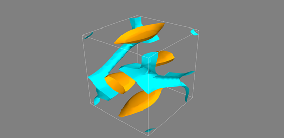
级数的等值面

import numpy as np
from mayavi.filters import mask_points
x,y,z = np.mgrid[0:1:20j,0:1:20j,0:1:20j]

u = np.sin(np.pi*x) * np.cos(np.pi*z)
v = -2*np.sin(np.pi*y) * np.cos(2*np.pi*z)
w = np.cos(np.pi*x)*np.sin(np.pi*z) + np.cos(np.pi*y)*np.sin(2*np.pi*z)

from mayavi import mlab
src = mlab.pipeline.vector_field(u,v,w)
# mlab.pipeline.vector_cut_plane(src, mask_points=10, scale_factor=2.0)
magnitude = mlab.pipeline.extract_vector_norm(src)
mlab.pipeline.iso_surface(magnitude, contours=[2.0,0.5])
mlab.outline()
mlab.show()

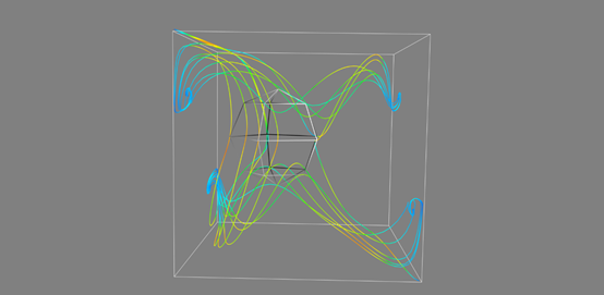
流线可视化

import numpy as np
from mayavi.filters import mask_points
x,y,z = np.mgrid[0:1:20j,0:1:20j,0:1:20j]

u = np.sin(np.pi*x) * np.cos(np.pi*z)
v = -2*np.sin(np.pi*y) * np.cos(2*np.pi*z)
w = np.cos(np.pi*x)*np.sin(np.pi*z) + np.cos(np.pi*y)*np.sin(2*np.pi*z)

from mayavi import mlab
# mlab.quiver3d(u,v,w)
# mlab.outline()
# mlab.show()

src = mlab.pipeline.vector_field(u,v,w)
# mlab.pipeline.vector_cut_plane(src, mask_points=10, scale_factor=2.0)
flow = mlab.flow(u,v,w,seed_scale=1,
                 seed_resolution=5,
                 integration_direction="both")

mlab.outline()
mlab.show()

矢量场复合观测

import numpy as np
from mayavi.filters import mask_points
from matplotlib.scale import scale_factory
x,y,z = np.mgrid[0:1:20j,0:1:20j,0:1:20j]

u = np.sin(np.pi*x) * np.cos(np.pi*z)
v = -2*np.sin(np.pi*y) * np.cos(2*np.pi*z)
w = np.cos(np.pi*x)*np.sin(np.pi*z) + np.cos(np.pi*y)*np.sin(2*np.pi*z)

from mayavi import mlab
# mlab.quiver3d(u,v,w)
# mlab.outline()
# mlab.show()
src = mlab.pipeline.vector_field(u,v,w)
magnitude = mlab.pipeline.extract_vector_norm(src)

iso = mlab.pipeline.iso_surface(magnitude,contours=[2.0,],opacity=0.3)
vec = mlab.pipeline.vectors(magnitude,mask_points=40,
                            line_width=1,
                            color=(0.8,0.8,0.8),
                            scale_factor=4.)
# mlab.pipeline.vector_cut_plane(src, mask_points=10, scale_factor=2.0)
flow = mlab.pipeline.streamline(
                 magnitude,
                 seedtype="plane",
                 seed_visible=False,
                 seed_scale=0.5,
                 seed_resolution=1,
                 linetype="ribbon")
vcp = mlab.pipeline.vector_cut_plane(magnitude,
                                     mask_points=2,
                                     scale_factor=4,
                                     colormap="jet",
                                     plane_orientation="x_axes")
mlab.outline()
mlab.show()

Ques:

1.标量数据和矢量数据分别使用什么方法进行绘制？

2.      2.矢量数据可视化实例中是如何对数据进行降采样的？

 

Answer:

1.  1.mlab.contour3d(x,y,z) and mlab.quiver3d(x,y,z)进行绘制

2.  2.Masking vector采样中的mlab.pipeline.vectors(src,mask_points=10,scale_factor=2.0)

4Mayavi三维可视化

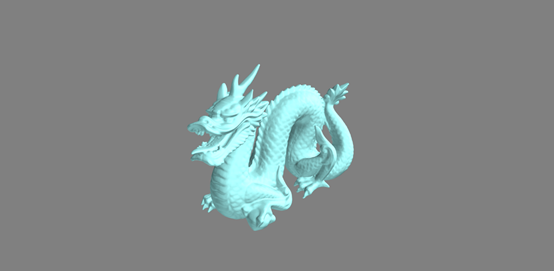
4.1绘制数据dragon

程序框架：

• 打开文件
• 使用modules绘制数据的surface
• 显示可交互的结果

渲染dragon ply文件：

from mayavi import mlab
import shutill #shutil可以中间删除显现的文件
mlab.pipeline.surface(mlab.pipeline.open(dragon_ply_file))
mlab.show()

代码例19

#coding=gbk
from os.path import join
from mayavi import mlab
import tarfile

#读取压缩文件内容
dragon_tar_file = tarfile.open("dragon.tar.gz")
try:
    os.mkdir("dragon_data")
except:
    pass
#将所有读取到的数据放入同一个文件夹中
dragon_tar_file.extractall("dragon_data")
dragon_tar_file.close()
#加入数据到dragon_ply_file中
dragon_ply_file = join("dragon_data","dragon_recon","dragon_vri.ply")

#渲染dragon.ply文件
mlab.pipeline.surface(mlab.pipeline.open(dragon_ply_file))
mlab.show()

#删除中间过程文件夹
import shutil
shutil.rmtree("dragon_data")

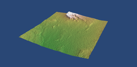
4.2绘制数据canyon

代码例20

#1_import packages
import zipfile
import numpy as np
from mayavi import mlab
# from pygame.examples.textinput import BGCOLOR
# from mayavi.tools.filters import warp_scalar

#2_hgt(Height File Format)
hgt = zipfile.ZipFile("N36W113.hgt.zip").read("N36W113.hgt")
# to certify a data type of integer,2X8=16 bit data
data = np.fromstring(hgt,">i2") 
# to certify the type of data
data.shape = (3601,3601) 
# to transform the type of data to 32bit
data = data.astype(np.float32)
# to increase the efficiency of showing, only choose sort of data
data = data[500:1000,500:1000]
#if there is any clearance in the source of data, set those to the minimum
data[data == -32768] = data[data > 0].min()

#3_use mlab.figure() to refresh the shape of the data and surf() to figure out the surface of the data
#the size of window with (400,320), background, color of shining upon, enlargement and contraction scale,
mlab.figure(size = (400,320),bgcolor=(0.16,0.28,0.46))
mlab.surf(data, colormap="gist_earth",warp_scale=0.2,vmin=1200,vmax=1610)

#4_clear the RAM for decomposition
del data

#5_create a window of Visualization, angle of position, height, distance
mlab.view(-5.9,83,570,[5.3,20,238])
mlab.show()

 

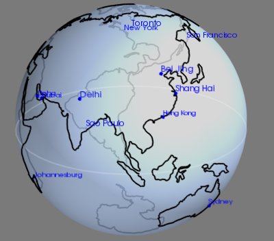
4.3绘制数据canyon

二维坐标如何转换成三维坐标？

x = R*cos(lat)*cos(lng);
y = R*cos(lat)*sin(lng);
z = R*sin(lat);
如果R = 1, 则
x = cos(lat)*cos(lng);
y = cos(lat)*sin(lng);
z = sin(lat);
lng表示经度，lat表示维度

代码例21

#get data of several cities and get their longitude as well as latitude)
from clyent import color
cities_data = """
Bei Jing, 116.23,39.54
Shang Hai, 121.52, 30.91
Hong Kong,114.19,22.38
Delhi,77.21,28.67
Johannesburg,28.04,-26.19
Doha,51.53,25.29
Sao Paulo,-46.63,-23.53
Toronto,-79.38,43.65
New York,-73.94,40.67
San Francisco,-122.45,37.77
Dubai,55.33,25.27
Sydney,151.21,-33.87
"""
# part2_create a list consisting of cities' indexes about their longtitudes and latitudes
import csv
#create a dict and a list
cities = dict()
coords = list()
# print(cities,coords)

# read data 
for line in list(csv.reader(cities_data.split("
")))[1:-1]:
    name, long_, lat = line
    cities[name] = len(coords)
    coords.append((float(long_),float(lat)))

# data transformation
import numpy as np
# from [1 line n row] to [n line, 1 list]
coords = np.array(coords)
# transform the angle to the arc
lat, long = coords.T * np.pi / 180
# transform 2D data to 3D data
# lat = ori_long
# long = ori_lat
x = np.cos(long) * np.cos(lat)
y = np.cos(long) * np.sin(lat)
z = np.sin(long)

#create a window
from mayavi import mlab
mlab.figure(bgcolor=(0.48,0.48,0.48), size=(400,400))

# to define a sphere
# set the opacity of the surface of earth to 0.7
sphere = mlab.points3d(0, 0, 0, scale_factor=2,
                       color = (0.67, 0.77, 0.93),
                       resolution = 50,
                       opacity = 0.7,
                       name = "Earth")

# to adjust the parameter of mirror reflection
sphere.actor.property.specular = 0.45
sphere.actor.property.specular_power = 5
# delete the opposite side to better show the effect of opacity
sphere.actor.property.backface_culling = True
# use points to describe sites of cities
points = mlab.points3d(x, y, z,
                       scale_mode = "none",
                       scale_factor = 0.03,
                       color = (0, 0, 1))

#create names of cities
# for cities.items output the names of cities and the series of cities 
for city, index in cities.items():
    #x,y,z mean x,y,z coordinates; color means text's color; width means text's width; name means text's object
    label = mlab.text(x[index], y[index], city,
                      z=z[index], color=(0,0,1),
                      width=0.016 * len(city), name=city)

#create continents
from mayavi.sources.builtin_surface import BuiltinSurface
continents_src = BuiltinSurface(source="earth", name="Continents")
#set the LDD to 2
continents_src.data_source.on_ratio = 2
continents = mlab.pipeline.surface(continents_src, color=(0,0,0))

#create the equitor
# distribute every 360 to 100
theta = np.linspace(0, 2 * np.pi, 50)
x = np.cos(theta)
y = np.sin(theta)
z = np.zeros_like(theta)
mlab.plot3d(x,y,z,color=(1,1,1),opacity=0.2,tube_radius=None)

#show the window for interation
mlab.view(100,60,4,[-0.05,0,0])
mlab.show()

5Mayavi三维可视化

5.1三维可视之基础应用homework1

pass见下文url

5.2三维可视之基础应用homework2

pass见下文url

5.3三维可视之基础应用homework3

pass见下文url

5.4三维可视之基础应用homework4

pass见下文url

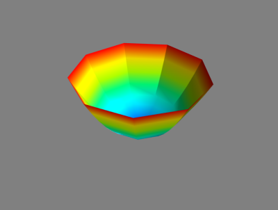
5.5三维可视之进阶实战homework5

构造一个旋转抛物面，并使用mlab.mesh绘制出来。首先在（r, theta）中创建一个20*20的二维网格：

r, theta = mgrid[0:1:10j, 0:2*pi:10j]

并将圆柱坐标系，转换为直角坐标系，其中：

z = r*r
x = r*cos(theta)
y = r*sin(theta)

（数学函数等值可从numpy中导出。）

代码例22

from mayavi import mlab
import numpy as np

pi = np.pi
cos = np.cos
sin = np.sin
mgrid = np.mgrid

r,theta = pi/250,pi/250
[r,theta] = np.mgrid[0:1:10j,0:2*pi:10j]

x = r * cos(theta)
y = r * sin(theta)
z = r * r

s = mlab.mesh(x,y,z)
mlab.show()

5.6三维可视之进阶实战homework6

对“编程练习8.1”中旋转抛物面方程进一步绘制，计算一个二维数组 s，并且把它传递给mesh()的scalars 参数。观察一下绘制结果的变化。其中 s = x*y*z. 同时，请绘制该旋转抛物面的轮廓线。

空间轮廓线可视化代码：

#coding=gbk
from mayavi import mlab
import numpy as np
from tvtk.api import tvtk
from tvtk.common import configure_input
from tvtkfunc import ivtk_scene, event_loop

pi = np.pi
cos = np.cos
sin = np.sin
mgrid = np.mgrid

r,theta = pi/250,pi/250
[r,theta] = np.mgrid[0:1:10j,0:2*pi:10j]

x = r * cos(theta)
y = r * sin(theta)
z = r * r
s = x * y * z
s = scalars
s = mlab.mesh(scalars,x,y,z)

plot3d = tvtk.MultiBlockPLOT3DReader(
        xyz_file_name="s",
        q_file_name="s",
        scalar_function_number=100, vector_function_number=200
    )#读入Plot3D数据
plot3d.update()#让plot3D计算其输出数据
grid = plot3d.output.get_block(0)#获取读入的数据集对象
outline = tvtk.StructuredGridOutlineFilter()#计算表示外边框的PolyData对象
configure_input(outline, grid)#调用tvtk.common.configure_input()
m = tvtk.PolyDataMapper(input_connection=outline.output_port)
a = tvtk.Actor(mapper=m)
a.property.color = 0.3, 0.3, 0.3
 
#窗口绘制
win = ivtk_scene(a)
win.scene.isometric_view()
event_loop()

mlab.show()

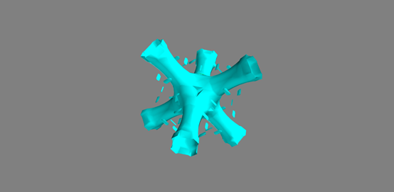
5.7三维可视之进阶实战homework7

可视化模型数据文件（附件），能发现了什么？

能发现一只白色雕塑的兔子

对于tar.gz类型压缩包的处理，可以参考dragon模型，可以参考以下代码：

#coding=gbk
from mayavi import mlab
from os.path import join
import tarfile

dragon_tar_file = tarfile.open("dragon.tar.gz")
try:
    os.mkdir("dragon_data")
except:
    pass
dragon_tar_file.extractall("dragon_data")
dragon_tar_file.close()
dragon_ply_file = join("dragon_data","dragon_recon","dragon_vrip.ply")

#渲染dragon ply文件
mlab.pipeline.surface(mlab.pipeline.open(dragon_ply_file))
mlab.show()

import shutil
shutil.rmtree("dragon_data")

大致逻辑如下：

选中并打开bunny.tar.gz---新建文件夹bunny_data---解压bunny.tar.gz到bunny_data文件夹---关闭bunny.tar.gz---串联路径从bun.zipper.ply（一般ply文件是最终目录下的扫描文件）到上一级再到上一级到最终建立的文件夹bunny_data---打开上面构建好的路径下的ply文件，用mlab.pipeline.surface()构建表面---用shutil.rmtree删除用于放置压缩文件的文件夹。

代码：

# 3D scanning files
from mayavi import mlab
from os.path import join
import tarfile

bunny_tar_file = tarfile.open("bunny.tar.gz")
try:
    os.mkdir("bunny_data")
except:
    pass
bunny_tar_file.extractall("bunny_data")
bunny_tar_file.close()
# combine the path of bun_vrip and its packages' name, such as dragon_data/dragon_recon/dragon_vrip.ply 
bunny_ply_file = join("bunny_data","bunny","reconstruction","bun_zipper.ply")

mlab.pipeline.surface(mlab.pipeline.open(bunny_ply_file))
mlab.show()

import shutil
shutil.rmtree("bunny_data")

补充：mlab绘图函数的x、y、z、s、w、u、v到底是什么含义？假设这些参数描述了一个磁场，它们可能分别代表什么含义?加入这些参数描述了一个流体，它们可能分别代表什么含义？

X,y,z表示点三维坐标；

S表示该坐标点处的标量值；

U,v,w表示矢量元素

如果应用到磁场中，x,y,z表示磁场位置，s表示该位置处磁场大小，u,v,w表示该处磁场方向。

如果应用到流体，x,y,z表示流体位置，s表示该处流量大小，u,v,w表示该处流量方向。

LOD：level of details

5.8三维可视之进阶实战homework8

1.为mayavi可视化提供数据的mayavi管线层级是Filters，这句话对吗？为什么？

不对，因为为mayavi可视化提供数据的是scence场景，scence每个场景下有多个数据集合sources，为mayavi可视化提供数据，Filter是应用于source上对数据进行变换。

2.基于1维Numpy数组x、y、z提供的三维坐标数据，绘制线图形的函数是Point3D()。这句话正确吗？为什么？

不对，因为基于1维Numpy数组x,y,z提供的三维坐标数据，绘制线图形的函数是plot3D(), point3d()是基于数组x,y,z提供的三维点坐标，绘制点图形。

3.mayavi管线中处于最顶层表示场景的对象是什么？获取当前场景的方法是什么？

Mayavi中处于最顶层的对象是mayavi Engine，表示建立和销毁场景Scene。

获取当前场景的方法是s.scene.background()

4.3D绘图函数Point3D()中，根据标量值确定actor透明度的参数是opcity。这句话正确吗？为什么？

不对，根据标量值确定actor透明度的参数是transparent，opcity用于VTK对象的整体透明度，该值为float型，默认为1.0

5.3D绘图函数中，绘制由三个二维数组x、y、z描述坐标点的网格平面的方法是imshow()。这句话正确吗？为什么？

不对，imshow()是用于绘制二维数组的，但是没有z轴，只有x和y两个轴，x作为第一轴的下标，y轴作为第二轴的下标

比如：s = numpy.random.random((10,10))，img = mlab.imshow(s,colormap='gist_earth')

6.3D绘图函数中，三维矢量数据的可视化的方法是contour3d()。这句话正确吗？为什么？

Contour3d是用来绘制标量数据3d视图的，三维矢量数据可视化的方法是mlab.quiver3d()。

7.在鼠标选取操作中，on_mouse_pick()方法返回值是什么？

On_mouse_pick()返回一个vtk对象。

8.mlab管线中，用来进行数据变换的层级是什么？用来实现数据可视化的层级是什么？

用filter对数据进行交换，用modules来对最终的数据进行可视化。

9.在mlab管线的modules层级中，用来对VTK dataset和mayavi sources建立外表面的方法是surface()。这句话正确吗？为什么？

正确，但是要却别与iso_surface(),iso_surface()是用于对输入的体数据绘制其等值面。

10.在mayavi可视化实例三中，绘制大洲边界时大洲边界粗糙的解决办法是什么？

调整LOD，比如调整continents_src.data_source.on_ratio = 2

6三维可视化之交互界面

6.1三维可视之进阶实战homework8

• Traits背景：
Python动编程态语言，变量没有类型，比如：颜色属性
“Red”字符创
0xff0000整数
（255，0,0）元组
• Traits库可以为python添加类型定义
• Traits属于解决color类型的问题
o 接受能表示颜色的各种类型值
o 赋值为非法的颜色值时，能够捕捉到错误，并给提供错误报告。
o 提供一个内部的标注你颜色
• c.color可以支持颜色命令，如c.color = “red”，但不支持c.color = “abc”的字符串
• c.configure_traits()可以设置颜色，c.color.getRgb()可以获取设置颜色后的三原色的值
比如设置c.configure_traits()为红色，即在桌面弹出的窗口中设置Red，那么回击c.color.getRgb可以得到(255,0,0,255)这样的feedback。 

6.2attributes of traits

traits的五个功能：initialization, verification, procuration, monitoring, visualization

代码23 traits

from traits.api import Delegate, HasTraits, Instance, Int, Str
 
class Parent(HasTraits):
    # 初始化
    last_name = Str('Zhang')
 
class Child(HasTraits):
    age = Int
    # 验证
    father = Instance(Parent)
    # 代理
    last_name = Delegate('father')
    # 监听
    def _age_changed(self, old, new):
        print('Age change from %s to %s' % (old, new))

练习过程如下：

>>> P = Parent()
>>> c = Child()
>>> c.father = P
>>> c.last_name
'Zhang'
>>> P.last_name
'Zhang'
>>> c.age = 4
Age changed from 0 to 4
>>> 
>>> c.configure_traits()
Age changed from 4 to 3
Age changed from 3 to 4
True
>>> c.print_traits()
age:       4
father:    <__main__.Parent object at 0x0000022BA2A2F8E0>
last_name: 'Zhang'
>>> c.get()
{'age': 4, 'father': <__main__.Parent object at 0x0000022BA2A2F8E0>, 'last_name': 'Zhang'}
>>> c.set(age = 8)
Age changed from 4 to 8
<__main__.Child object at 0x0000022BA2A2F990>

在traits属性功能的实例中，能否直接修改Child的last_name属性？

不能，因为Child对象的last_name是直接继承自Parent类的，要通过父类改变

如果定义P = Parent(), c = Child();

直接输出c.last_name 没有结果

所以输出c.father = P, 再输入c.last_name就有子类名字

或者也可以直接输入P.last_name也可以得到子类名字

6.3traits属性监听

Trait属性监听：静态监听，动态监听

Trait监听属性顺序：name, age, doing---静态监听函数---动态监听1---动态监听2

静态监听函数的几种形式：属性名+changed+发生变化前的名+发生变化后的名字

_age_changed(self)
_age_changed(self,new)
_age_changed(self, old, new)
_age_changed(self, name, old, new)

动态监听：

@on_trait_change(names)
Def any_method_name(self, ..)

 

问：为什么对Infoupdated任意赋值都会触发监听事件？

因为Infoupdated直接由Event赋值，无论如何都会调用_Infoupdated_fired()函数，所以会触发self.reprint()函数输出self.name和self.age内容。

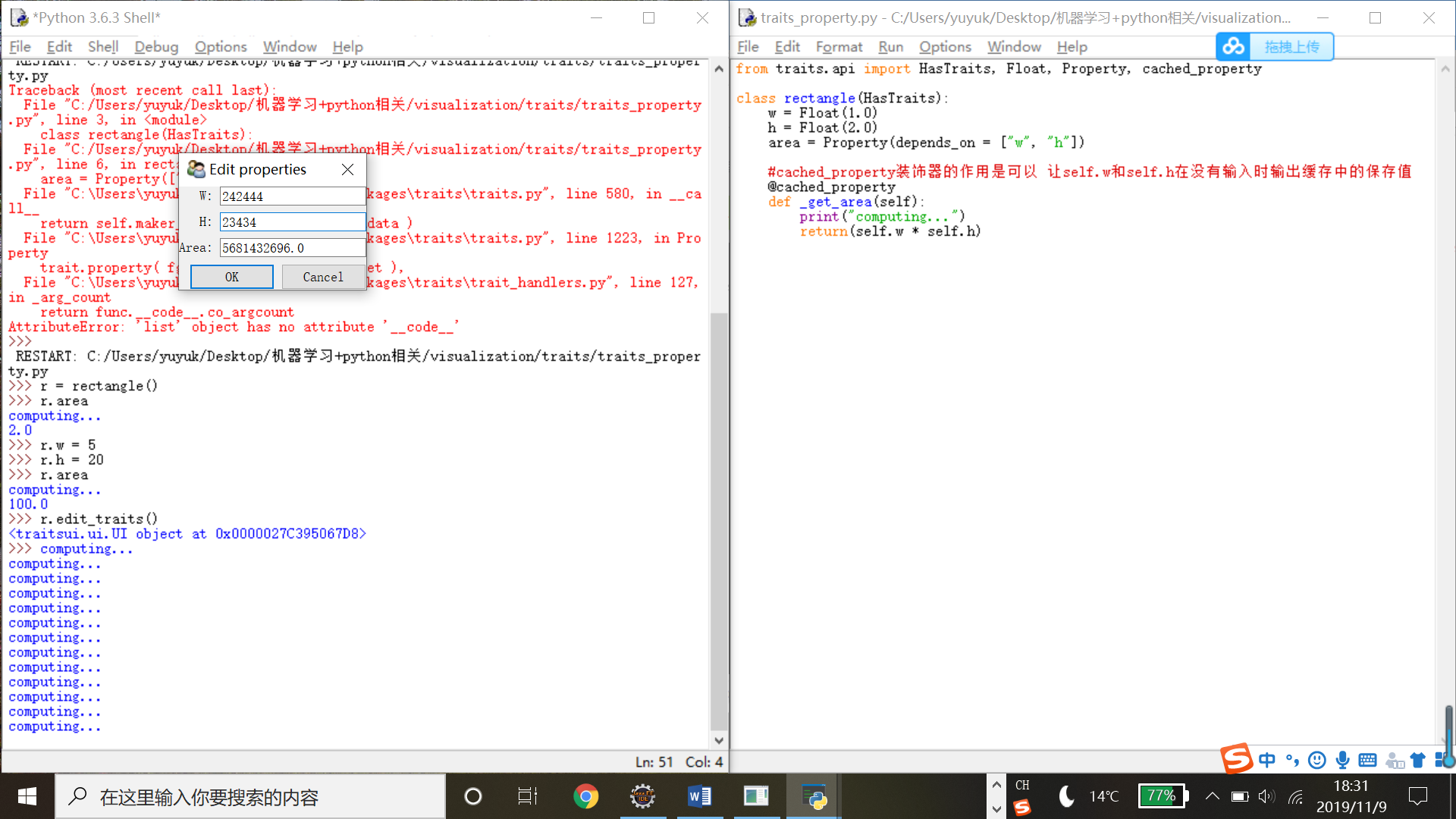
6.5Traits_property

用traits_property.py遍好程序后，得到area被监听的结果；如果命令行输入w/h发生变化，print输出的就是变化后的值。

调用r.edit_traits()直接触发_get_area()函数，同时在界面中显示area结果。

6.6TraitsUI

Tkinter, wxPython, pyQt4, TraitsUI(based on MVC：Model-View-Controller)

MVC是traitsUI所使用的架构模型

6.6.1Traits_UI交互

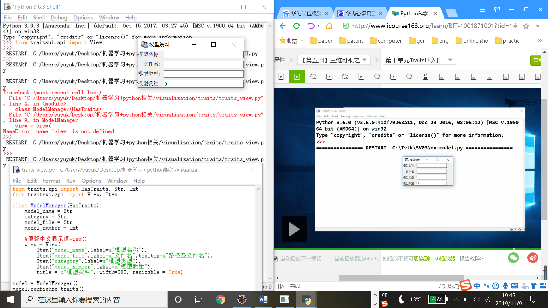
from traits.api import HasTraits, Str, Int
class ModelManager(HasTraits):
    model_name = Str
    category = Str
    model_file = Str
    model_number = Int
model = ModelManager()
model.configure_traits()

6.6.2View定义界面

TraitsUI自定义界面支持的后台库界面有：qt4(-toolkit qt4)和wx(-toolkit wx)

MVC类别	MVC说明
Model	HasTraits的派生类用Trait保存数据，相当于模型
View	没有指定界面显示方式时，Traits自动建立默认界面
Controller	起到视图和模型之间的组织作用，控制程序的流程

•Item对象属性

Item(id,name,label)

属性	说明
id	Item的唯一ID
name	Trait属性的名称
Label	静态文本，用于显示编辑器的标签
Tooltip	编辑器的提示文本

•View对象属性

属性	说明
Title	窗口标题栏
Width	窗口高度
Height	串口高度
Resizable	串口大小可变，默认为True

代码和界面如下：

问：如果想要编辑器窗口大小不能改变，应如何修改view中的哪个属性？

答：修改title中的resizable = False可以是标签大小不可变

6.6.3Group组织对象

Group对象

from traitsui.api import Group

Group(…)属性有：

属性	说明
Orientation	编辑器的排列方向
Layout	布局方式normal,flow,split,tabbed
Show_labels	是否显示编辑器的标签
Columns	布局的列数，范围为（1,50）

·       Group类继承的HSplit类

Hsplit定义：
Class HSplit(Group):
    #...
    #...
    Layout = “split”
    Orientation = “horizontal”

代码等价于：

Group(…, layout = “split”, orientation = “horizontal”)

•Group的各种派生类

属性	说明
HGroup	内容水平排列 Group(orientation = “horizontal”)
HFlow	内容水平排列，超过水平宽度，自动换行，隐藏标签文字。Group(orientation = “horizontal”, layout=”flow”, show_labels = False)
HSplit	内容水平分隔，中间插入分隔条
Tabbed	内容分标签页显示 Group(orientation=”horizontal”,layout=”tabber”)
Vgroup	内容垂直排列 Group(orientation=”vertical”)
Vflow	内容垂直排列，超过垂直高度时，自动换列，隐藏标签文字Group(orientation=”vertical”,layout=”flow”,show_labels=False)
Vfold	内容垂直排列，可折叠 Group(orientation=”vertical”,layout=”fold”,show_labels=False)
Vgrid	按照多列网格进行垂直排列，columns属性决定网格的列数 Group(orientation=”vertical”,columns=2)
Vsplit	内容垂直排列，中间插入分隔条 Gorup(orientation=”vertical”,layout=”split”)

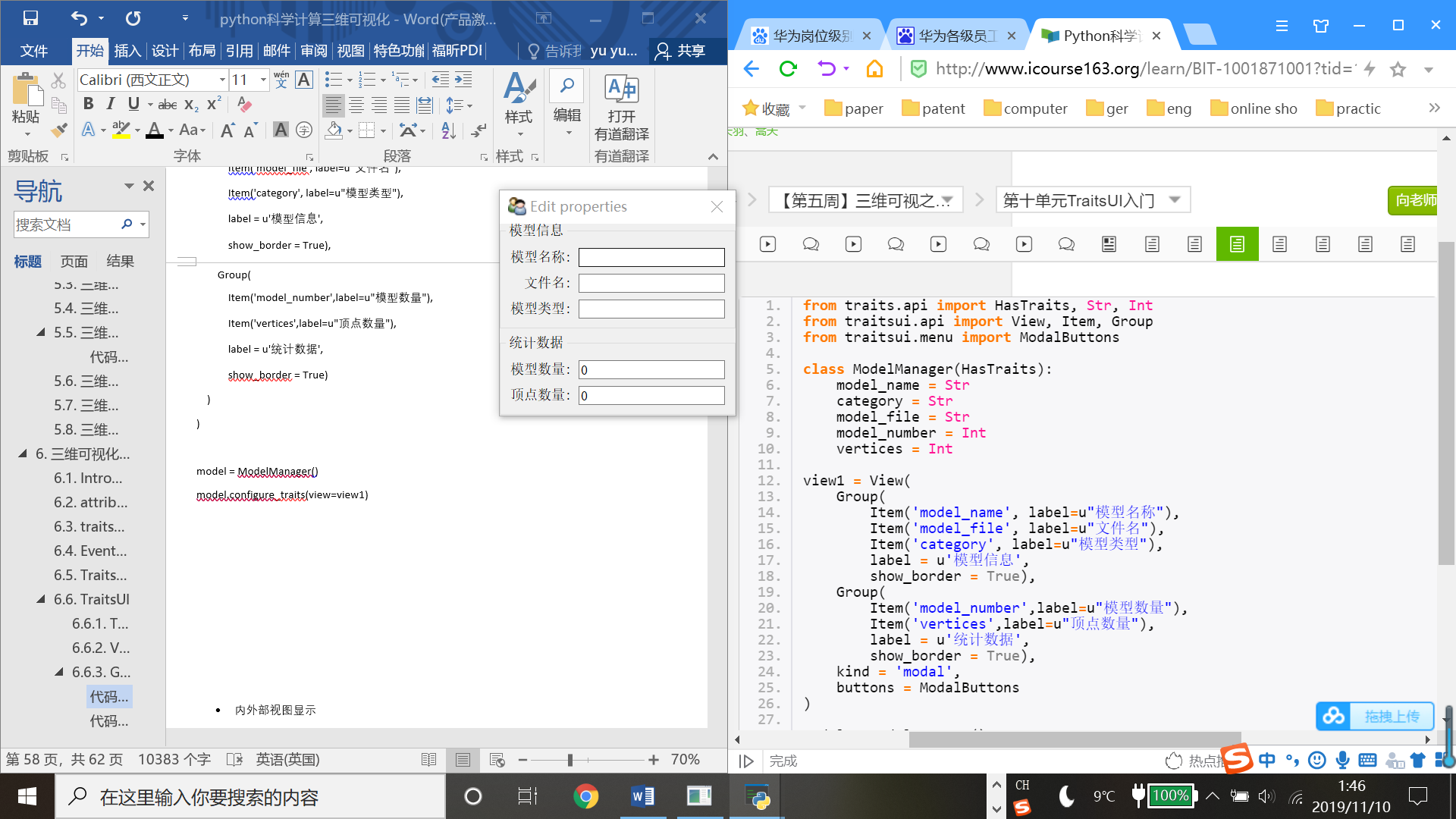
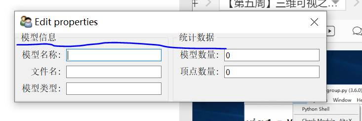
代码24  多视图界面代码

from traits.api import HasTraits, Str, Int
from traitsui.api import View, Item,Group
from traitsui.menu import ModalButtons

class ModelManager(HasTraits):
    model_name = Str
    category = Str
    model_file = Str
    model_number = Str
    vertices = Int

view1 = View(
    Group(
        Item("model_name",label=u"模型名称"),
        Item("model_name",label=u"文件名"),
        Item("category",label=u"模型类型"),
        label = u"模型信息",
        show_border = True),
    Group(
        Item("model_number",label=u"模型数量"),
        Item("vertices",label=u"顶点数量"),
        label = u"统计数据",
        show_border = True),
    kind = "modal",
    buttons = ModalButtons
)

model = ModelManager()
model.configure_traits(view=view1)

•垂直排列多视图

from traits.api import HasTraits, Str, Int
from traitsui.api import View, Item, Group
from traitsui.menu import ModalButtons
 
class ModelManager(HasTraits):
    model_name = Str
    category = Str
    model_file = Str
    model_number = Int
    vertices = Int
 
view1 = View(
    Group(
        Group(
            Item('model_name', label=u"模型名称"),
            Item('model_file', label=u"文件名"),
            Item('category', label=u"模型类型"),
            label = u'模型信息',
            show_border = True),
        Group(
            Item('model_number',label=u"模型数量"),
            Item('vertices',label=u"顶点数量"),
            label = u'统计数据',
            show_border = True)
    )
)
    
model = ModelManager()
model.configure_traits(view=view1)

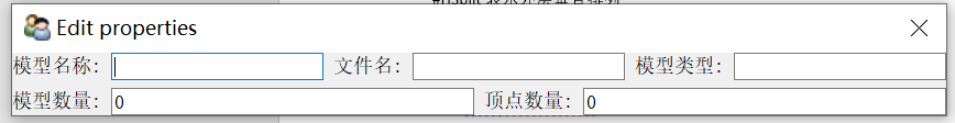
•水平排列多视图

from traits.api import HasTraits, Str, Int
from traitsui.api import View, Item, Group
from traitsui.menu import ModalButtons
 
class ModelManager(HasTraits):
    model_name = Str
    category = Str
    model_file = Str
    model_number = Int
    vertices = Int
 
view1 = View(
    Group(
        Group(
            Item('model_name', label=u"模型名称"),
            Item('model_file', label=u"文件名"),
            Item('category', label=u"模型类型"),
            label = u'模型信息',
            show_border = True),
        Group(
            Item('model_number',label=u"模型数量"),
            Item('vertices',label=u"顶点数量"),
            label = u'统计数据',
            show_border = True),
        orientation = "horizontal"
    )
)
    
model = ModelManager()
model.configure_traits(view=view1)

•Hsplit和VGroup定义水平/垂直并排视图

同样也可以用HSplit和VGroup去生成水平/垂直排列

from traits.api import HasTraits, Str, Int
from traitsui.api import View, Item, VGroup, HSplit
from traitsui.menu import ModalButtons
 
class ModelManager(HasTraits):
    model_name = Str
    category = Str
    model_file = Str
    model_number = Int
    vertices = Int
 
view1 = View(
    #HSplit表示外层垂直排列
    HSplit(
        VGroup(
            Item('model_name', label=u"模型名称"),
            Item('model_file', label=u"文件名"),
            Item('category', label=u"模型类型"),
            label = u'模型信息'),
        VGroup(
            Item('model_number',label=u"模型数量"),
            Item('vertices',label=u"顶点数量"),
            label = u'统计数据')
    )
)
    
model = ModelManager()
model.configure_traits(view=view1)

•  外层垂直排列

from traits.api import HasTraits, Str, Int
from traitsui.api import View, Item, HGroup, VSplit
from traitsui.menu import ModalButtons
 
class ModelManager(HasTraits):
    model_name = Str
    category = Str
    model_file = Str
    model_number = Int
    vertices = Int
 
view1 = View(
    #HSplit表示外层垂直排列
    VSplit(
        HGroup(
            Item('model_name', label=u"模型名称"),
            Item('model_file', label=u"文件名"),
            Item('category', label=u"模型类型"),
            label = u'模型信息'),
        HGroup(
            Item('model_number',label=u"模型数量"),
            Item('vertices',label=u"顶点数量"),
            label = u'统计数据')
    )
)
    
model = ModelManager()
model.configure_traits(view=view1)

• 内外部视图显示

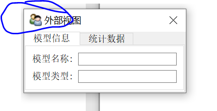
• 代码25

from traits.api import HasTraits, Str, Int
from traitsui.api import View, Item,Group
from traitsui.menu import ModalButtons

g1 = [Item("model_name", label=u"模型名称"),
      Item("category", label=u"模型类型")]
g2 = [Item("model_number", label=u"模型数量"),
      Item("vertices", label=u"顶点数量")]
class ModelManager(HasTraits):
    model_name = Str
    category = Str
    model_file = Str
    model_number = Str
    vertices = Int
    traits_view = View(
        Group(*g1, label = u"模型信息", show_border = True),
        Group(*g2, label = u"统计数据", show_border = True),
        title = u"内部视图")
global_view = View(
    Group(*g1, label = u"模型信息", show_border = True),
    Group(*g2, label = u"统计数据", show_border = True),
    title = u"外部视图")

model = ModelManager()

• 在命令行输入不同代码出现不同界面：

>>> model.configure_traits(view = global_view)

>>> model.configure_traits()

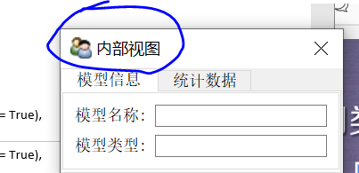
>>> model.configure_traits(view = "traits_view")

如果想要在编辑器中水平并列显示三组group对象

Q1.如果想要在编辑器中水平并列显示三组group对象，应该如何修改group对象的属性？

A1.把原来的Group()改成HGroup()或者在列完3个内层Group同级上写orientation = “horizontal”

Q2.如果想要在编辑器中垂直分标签页显示若干组group对象，可以使用哪些方法？

同理把原来的Group()改成VGroup()或者在列完若干个内层Group()同级上写orientation = “vertical”

6.6.4视图配置

通过kind属性设置view显示类型

显示类型	说明
Modal	模态窗口，非即时更新
Live	非模态窗口，即时更新
Livemodal	模态窗口，即时更新
Nonmodal	非模态窗口，非即时更新
Wizard	向导类型
Panel	嵌入到其他窗口中的面板，即时更新，非模式
Subpanel

显示类型（采用窗口显示内容）

Modal

Live

Livemodal

nonmodal

模态窗口：在窗口关闭之前，其他窗口不能激活；

无模态窗口：在窗口关闭之前，其他窗口能激活；

即时更新：修改空间内容，立即反映到模型数据上；

非即时更新：只有当用户点ok，apply等命令时，效果才会反应在模型上；

Wizard：向导窗口，模态窗口，即时更新；

Panel：向导窗口，模态窗口，即时更新

subpanel ：嵌入窗口中的面板

视图配置的实例：view = view(… kind = ‘modal=’)

模态与非模态的小例子

Configure_traits	Edit_traits()
界面显示后，进入消息循环	界面显示后，不进入消息循环
主界面窗口或模态对话框	无模态窗口或对话框

Traits UI按钮配置

标准命令按钮

UndoButton

Applybutton

ReverButton

OKbutton

CancelButton

HelpButton

Traitsui.menu预定义了命令按钮：
OKcancelButtons = [OKButton,CancelButton]
ModelButtons = [ApplyButton,RevertButton,OKButton,CancelButton,HelpButton]
LiveButtons = [UndoButton,ReverButton,OKButton,Cancel]

6.6.5TraitsUI控件

文本编译器：Str, Int

文本编译器与密码窗口：

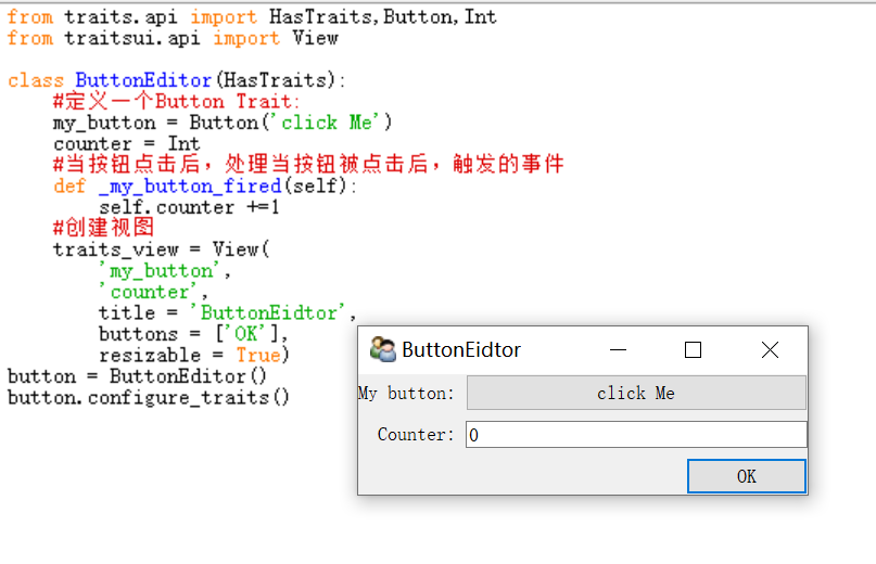
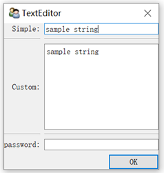
from traits.api import HasTraits, Str, Password
from traitsui.api import Item, Group, View

class TextEditor(HasTraits):
    #定义文本编辑器变量
    string_trait = Str('sample string')
    password = Password
    #定义布局
    text_str_group = Group(
        Item('string_trait',style = 'simple',label = 'Simple'),
        Item("_"),
        Item('string_trait',style = 'custom',label = 'Custom'),
        Item("_"),
        Item('password',style = 'simple',label = 'password'),
        )
    #定义视图
    traits_view = View(
        text_str_group,
        title = 'TextEditor',
        buttons = ['OK']
        )
代码25  按键触发计数器
from traits.api import HasTraits,Button,Int
from traitsui.api import View

class ButtonEditor(HasTraits):
    #定义一个Button Trait:
    my_button = Button('click Me')
    counter = Int
    #当按钮点击后，处理当按钮被点击后，触发的事件
    def _my_button_fired(self):
        self.counter +=1
    #创建视图
    traits_view = View(
        'my_button',
        'counter',
        title = 'ButtonEidtor',
        buttons = ['OK'],
        resizable = True)
button = ButtonEditor()
button.configure_traits()

代码26 滑动条

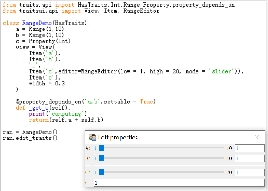
from traits.api import HasTraits,Int,Range,Property,property_depends_on
from traitsui.api import View, Item, RangeEditor

class RangeDemo(HasTraits):
    a = Range(1,10)
    b = Range(1,10)
    c = Property(Int)
    view = View(
        Item('a'),
        Item('b'),
        '_',
        Item('c',editor=RangeEditor(low = 1, high = 20, mode = 'slider')),
        Item('c'),
        width = 0.3
    )

    @property_depends_on('a,b',settable = True)
    def _get_c(self):
        print('computing')
        return(self.a + self.b)

ran = RangeDemo()
ran.edit_traits()

text = TextEditor()
text.configure_traits()

按钮Button Editor
监听方法: _TraitName_fired()
TraitName是Button Trait 的名字，即my_button
Def _my_button_fired(self):
    Self.counter += 1

程序框架：

from traits.api import Button #导入控件模块
class ButtonEditor(HasTraits):
    TraitName = Button() #定义按钮变量名
    def _TraitName_fired(self) #定义监听函数
       … …
    view = View()
button = Button()
button.configure_traits()

菜单、工具栏

From traitsui.menu import Action…

对象	说明
Action	在Menu对象中，通过Action对象定义菜单中的每个选项
ActionGroup	在菜单中的选项中进行分组
Menu	定义菜单栏中的一个菜单
MenuBar	菜单栏对象，由多个Menu对象组成
ToolBar	工具栏对象，它由多个Action对象组成，每个Aciton对应工具挑中的一个按钮

fdf控件列表

 

对象	说明
Array	数组空间
Bool	单选框、复选框
Button	按钮
Code	代码编辑器
Color	颜色对话框
Directory	目录控件
Enum	枚举控件
File	文件控件
Font	字体选择控件
Html	Html网页控件
List	列表框
Str	文本框
Password	密码控件
Tuple	元组控件

 

7三维可视化之界面实战

7.1TraitsUI与mayavi实战

7.1.1Mayavi可视化实例

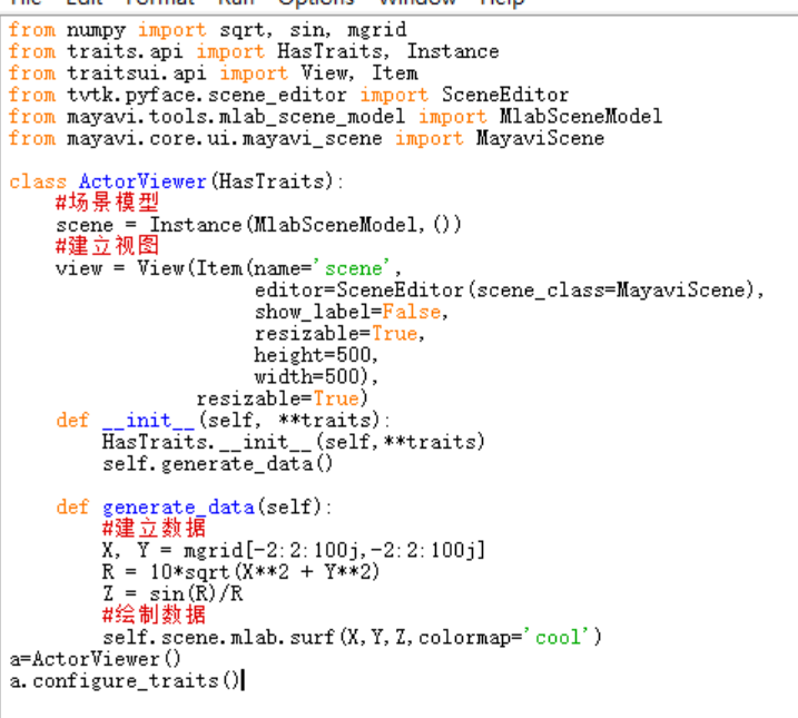
建立mayavi窗口步骤：
　　1. 建立从HasTraits继承的类
　　　　a. 建立MlabSceneMode场景实例scene
　　　　b. 建立view视图
　　　　c. 定义_init_函数，生成数据
　　2. 建立类的实例，调用configure_traits()方法

Numpy                                            　　用于建立数据

Traits.api，traitsui.api                 　　    用于建立场景模型

Tvtk.pyface.scene_editor            　　   用于建立视图

Tools.mlab_scene_model          　　     用于绘制数据

Core.ui.mayavi_scene                  　　  用于绘制数据

7.1.2TraitsUI可视化实例

程序框架

#1.定义HasTraits继承类

Class MyModel(HasTraits):
#1.1定义窗口的变量
n_meridional
n_longitudinal
scene
#1.2更新视图绘制
@on_trait_change()
Def update_plot(self):
    … …
#1.3建立视图布局
View = View()

#2.显示窗口

model = MyModel()
Model.configure_traits()

7.1.3三维可视之交互界面homework6

pass见下文url

8三维可视化之总结

8.1客观题练习homework7

pass见下文url

8.2主观题练习

8.2.1练习1

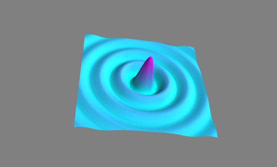
请参考SV11V02“TraitsUI可视化实例”，将本课程所学的TVTK或者Mayavi可视化例子，补充TraitsUI的交互控制，即通过TraitsUI的交互控制能够实现可视化视图中参数的相应改变，交互控件的种类不少于2种（如滑动条、文本框）、交互控件数量不少于3个（如2个滑动条、1个文本框）。要求代码规范，有注释。

SV11V02 TraitsUI可视化实例参考代码

一个简单的例子，在原有基础上，融合了文本框和[‘OK’]按钮

from traits.api import HasTraits, Range, Instance, on_trait_change
from traitsui.api import View, Item, Group
from mayavi.core.api import PipelineBase
from mayavi.core.ui.api import MayaviScene, SceneEditor, MlabSceneModel

from numpy import arange, pi, cos, sin
dphi = pi/300.
phi = arange(0.0, 2*pi + 0.5*dphi, dphi, 'd')
def curve(n_mer, n_long):
    mu = phi*n_mer
    x = cos(mu) * (1 + cos(n_long * mu/n_mer)*0.5)
    y = sin(mu) * (1 + cos(n_long * mu/n_mer)*0.5)
    z = 0.5 * sin(n_long*mu/n_mer)
    t = sin(mu)
    return x, y, z, t
 
class MyModel(HasTraits):
    n_meridional    = Range(0, 30, 6)
    n_longitudinal  = Range(0, 30, 11)
    # 场景模型实例
    scene = Instance(MlabSceneModel, ())
    # 管线实例
    plot = Instance(PipelineBase)
    #当场景被激活，或者参数发生改变，更新图形
    @on_trait_change('n_meridional,n_longitudinal,scene.activated')
    def update_plot(self):
        x, y, z, t = curve(self.n_meridional, self.n_longitudinal)
        if self.plot is None:#如果plot未绘制则生成plot3d
            self.plot = self.scene.mlab.plot3d(x, y, z, t,
                        tube_radius=0.025, colormap='Spectral')
        else:#如果数据有变化，将数据更新即重新赋值
            self.plot.mlab_source.set(x=x, y=y, z=z, scalars=t)
 
    # 建立视图布局
    view = View(Item('scene', editor=SceneEditor(scene_class=MayaviScene),
                     height=250, width=300, show_label=False),
                Group('_', 'n_meridional', 'n_longitudinal'),
                resizable=True)
 
model = MyModel()
model.configure_traits()

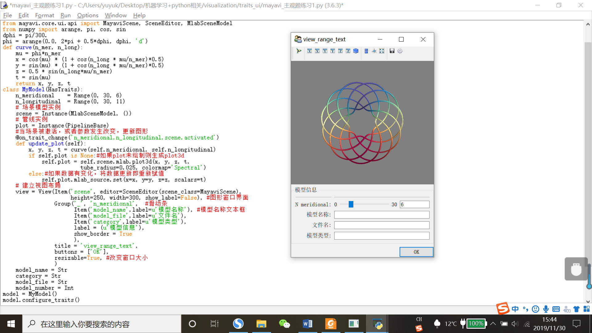
代码27 view_range_text

from traits.api import HasTraits, Range, Instance, on_trait_change, Str, Int, Button
from traitsui.api import View, Item, Group
from mayavi.core.api import PipelineBase
from mayavi.core.ui.api import MayaviScene, SceneEditor, MlabSceneModel
from numpy import arange, pi, cos, sin
dphi = pi/300.
phi = arange(0.0, 2*pi + 0.5*dphi, dphi, 'd')
def curve(n_mer, n_long):
    mu = phi*n_mer
    x = cos(mu) * (1 + cos(n_long * mu/n_mer)*0.5)
    y = sin(mu) * (1 + cos(n_long * mu/n_mer)*0.5)
    z = 0.5 * sin(n_long*mu/n_mer)
    t = sin(mu)
    return x, y, z, t
class MyModel(HasTraits):
    n_meridional    = Range(0, 30, 6)
    n_longitudinal  = Range(0, 30, 11)
    # 场景模型实例
    scene = Instance(MlabSceneModel, ())
    # 管线实例
    plot = Instance(PipelineBase)
    #当场景被激活，或者参数发生改变，更新图形
    @on_trait_change('n_meridional,n_longitudinal,scene.activated')
    def update_plot(self):
        x, y, z, t = curve(self.n_meridional, self.n_longitudinal)
        if self.plot is None:#如果plot未绘制则生成plot3d
            self.plot = self.scene.mlab.plot3d(x, y, z, t,
                        tube_radius=0.025, colormap='Spectral')
        else:#如果数据有变化，将数据更新即重新赋值
            self.plot.mlab_source.set(x=x, y=y, z=z, scalars=t)
    # 建立视图布局
    view = View(Item('scene', editor=SceneEditor(scene_class=MayaviScene),
                     height=250, width=300, show_label=False), #图形窗口界面
                Group('_', 'n_meridional',  #滑动条
                      Item('model_name',label=u'模型名称'), #模型名称文本框
                      Item('model_file',label=u'文件名'),
                      Item('category',label=u'模型类型'),
                      label = (u'模型信息'),                     
                      show_border = True
                      ), 
                title = 'view_range_text',
                buttons = ['OK'],
                resizable=True, #改变窗口大小
                )
    model_name = Str
    category = Str
    model_file = Str
    model_number = Int
model = MyModel()
model.configure_traits()

参考SV09V02“TraitsUI可视化实例”，将本课程所学的TVTK或者Mayavi可视化例子，补充TraitsUI的交互控制，即通过TraitsUI的交互控制能够实现可视化视图中参数的相应改变，交互控件的种类不少于3种（如滑动条、文本框、颜色对话框）、交互控件数量不少于3个（如1个滑动条、1个文本框、1个颜色对话框）。要求代码规范，有注释。

8.2.2练习2

SV09V02“TraitsUI可视化实例”参考代码：

from traits.api import Delegate, HasTraits, Instance, Int, Str

class Parent(HasTraits):
    # 初始化
    last_name = Str('Zhang')
 
class Child(HasTraits):
    age = Int
    # 验证
    father = Instance(Parent)
    # 代理
    last_name = Delegate('father')
    # 监听
    def _age_changed(self, old, new):
        print('Age change from %s to %s' % (old, new))

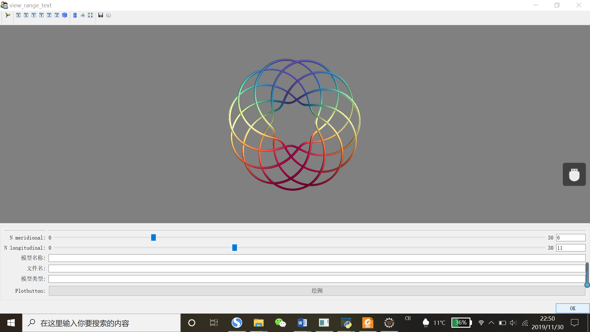
代码28 在TraitsUI中嵌入mayavi

颜色对话框没有找到，不会实现这个功能，不过添加了一个点击绘图的命令，代码稍微修改了下，添加了_plotbutton_fired(self)和plot(self)函数，同时在绘图之前要给图形一个初始化，在出现图形界面后，再动态监听图形参数的变化

# -*- coding: utf-8 -*-
from traits.api import *
from traits.api import HasTraits, Range, Instance, on_trait_change, Str, Int, Button
from traitsui.api import View, Item, VGroup,Group
from mayavi.core.api import PipelineBase
from mayavi.core.ui.api import MayaviScene, SceneEditor, MlabSceneModel
from numpy import arange, pi, cos, sin

dphi = pi/300.
phi = arange(0.0, 2*pi + 0.5*dphi, dphi, 'd')
def curve(n_mer, n_long):
    mu = phi*n_mer
    x = cos(mu) * (1 + cos(n_long * mu/n_mer)*0.5)
    y = sin(mu) * (1 + cos(n_long * mu/n_mer)*0.5)
    z = 0.5 * sin(n_long*mu/n_mer)
    t = sin(mu)
    return x, y, z, t

class DemoApp(HasTraits):
    n_meridional    = Range(0, 30, 6)
    n_longitudinal  = Range(0, 30, 11)
    plotbutton = Button(u"绘图")
    # 场景模型实例
    scene = Instance(MlabSceneModel,())
    #当场景被激活，或者参数发生改变，更新图形
    @on_trait_change('n_meridional,n_longitudinal,scene.activated')
    def update_plot(self): 
        x, y, z, t = curve(self.n_meridional, self.n_longitudinal)
        if self.plot is None:#如果plot未绘制则生成plot3d
            self.plot = self.scene.mlab.plot3d(x, y, z, t,
                        tube_radius=0.025, colormap='Spectral')
        else:#如果数据有变化，将数据更新即重新赋值
            self.plot.mlab_source.set(x=x, y=y, z=z, scalars=t)
    
    #建立视图
    view = View(
                Item('scene', editor=SceneEditor(scene_class=MayaviScene),height=250, width=300,show_label=False), #图形窗口界面
                Group('_','n_meridional','n_longitudinal',
                    Item('model_name',label=u'模型名称'),
                    Item('model_file',label=u'文件名'),
                    Item('category',label=u'模型类型'),
                    'plotbutton',
                    show_border = True
                    ), 
                title = 'view_range_text',
                buttons = ['OK'],
                resizable=True, #可变窗口大小
                )

    def _plotbutton_fired(self):
        self.plot()
        
    def plot(self):
        # 管线实例,初始化函数
        plot = Instance(PipelineBase)
        x, y, z, t = curve(self.n_meridional, self.n_longitudinal)
        self.plot = self.scene.mlab.plot3d(x, y, z, t,tube_radius=0.025, colormap='Spectral')
        
    model_name = Str
    category = Str
    model_file = Str
    
app = DemoApp()
app.configure_traits()

本博客中能提供到的

1.pdfhomework文本和答案；

2.部分数据集代码，如果选哟全部数据集，最好还是取中国MOOC顶部的url课程链接中下载，资料全；

3.关于这个课程，我做过编程训练的代码

4.pdf课程笔记。

github地址：here，上面对应的资料都在里面，不专业，不过代码都走了一遍，有些问题也想了下，供参考。

关于如何git上传，转一下这个大佬帖子，here

简单老说就是以下几个步骤：

1）.在github中创建好新的repository，如下图，其次就是命名，其他默认即可。

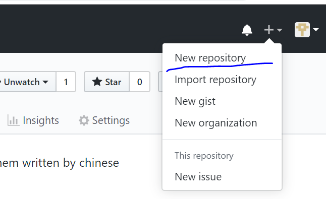
2）.把要上传的文件装在一个文件夹下；

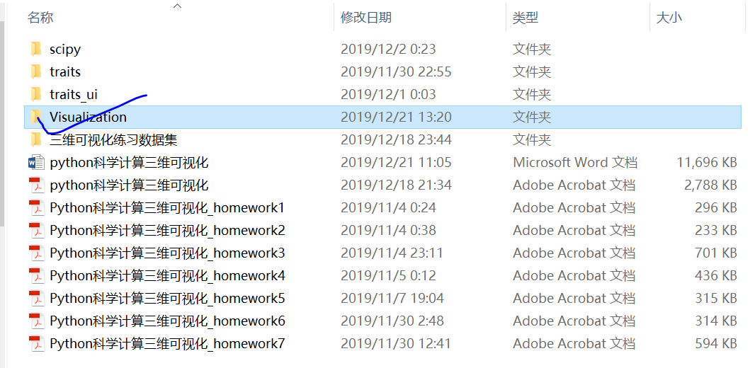
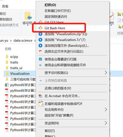
3）.右击这个文件夹，会出现git Bash和git GUI这个命令，点击git Bash（前提是已经装好了git)；

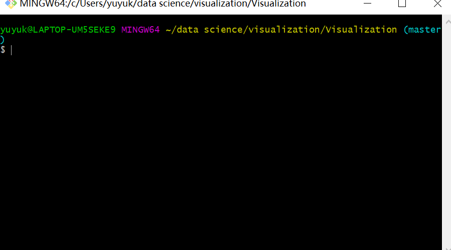
4）.进入git Bash后，是这个界面

5）.刚才创建好的repository里，复制链接

6）.截下来在git Bash中输入下面命令

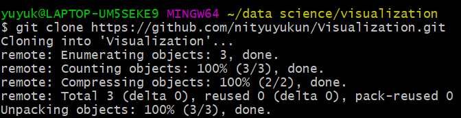
a）git clone xxxx(刚才复制的地址)，此时在本地要上传的文件夹里会多出一个文件夹（同文件名github中，创建的repository)，比如我是Visualization；

　  e.g. git clone https://github.com/nityuyukun/Visualization.git

b）.切换到本地仓库的文件夹，比如Visualiazation

c）git add .   //注意add后有一个空格，再加点，加点表示上传所有文件到本地仓库；

d）git commit -m "xxx"  //"xxx"中的xxx可以任意替换，表示想要备注的名字，比如我下面是second commit，这一步表示确认上传所有文件到本地仓库，并备份；

这两步完后，出现下图

e）git push -u origin master 这一步表示把本地仓库里的东西推到github上。

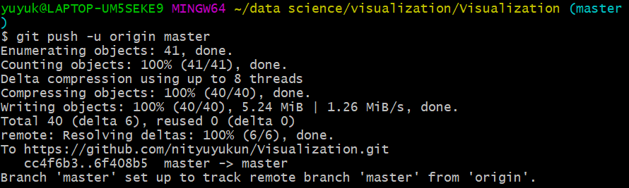
finished.