week4 neural networks I
4.1definitions of neural networks
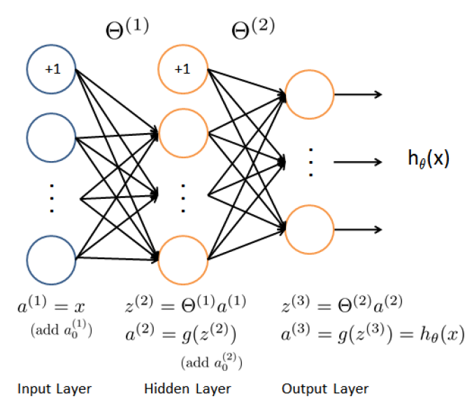
4.1.1dimensions of neural networks(how to define the hypothesis of neural networks)

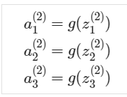
input层(层1)有3个神经元,隐藏层(层2)有4个神经元,那么这个矩阵是S2x(S1+1),计算:层1为3个neutrons,层2有4个neutrons。
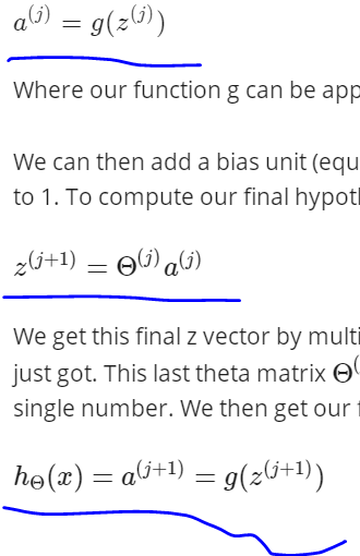
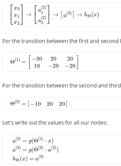
重新定义z函数,压缩到h函数中

神经网络中的真值表
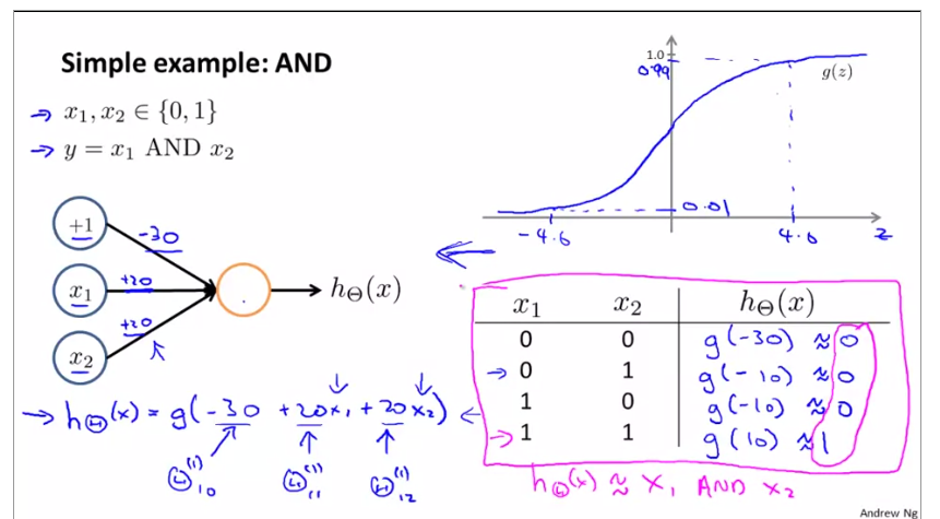
4.1.2application of Neutral networks
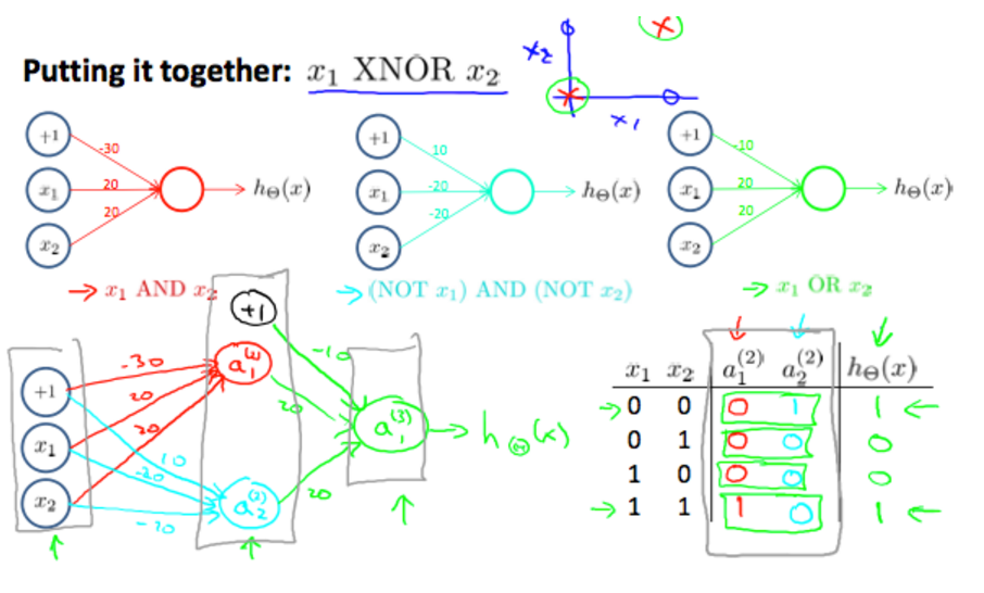
XNOR operator using a hidden layer((X1 XNOR X2) = ((X1 AND X2) AND ((NOT X1) AND (NOT X2)) AND (X1 OR X2)))
模型的输入与输出
4.2homeworkweek04
4.2.1载入数据集
load('ex3data1.mat'); % training data stored in arrays X, y
载入数据集运行后,可以得到如下手写数字集

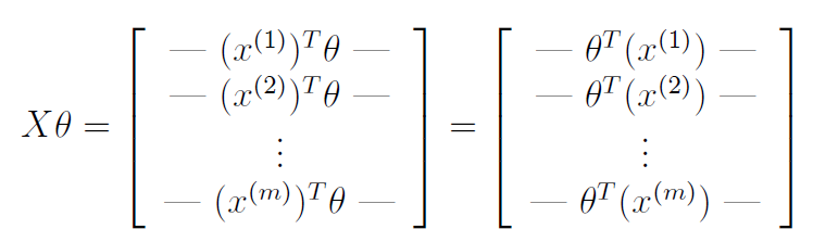
in the process of vectorization, we can use the equation that is aTb=bTa, so
week5 neural networks II
5.1the difference of cost function between logistic regression and neural networks
5.2the algorithm of optimization for cost function
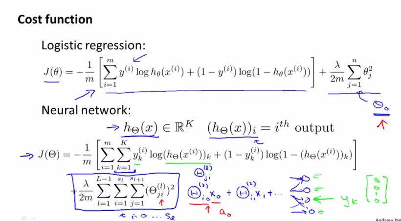
the cost function for regularized logistic regression is
![]()
for neural networks, it is

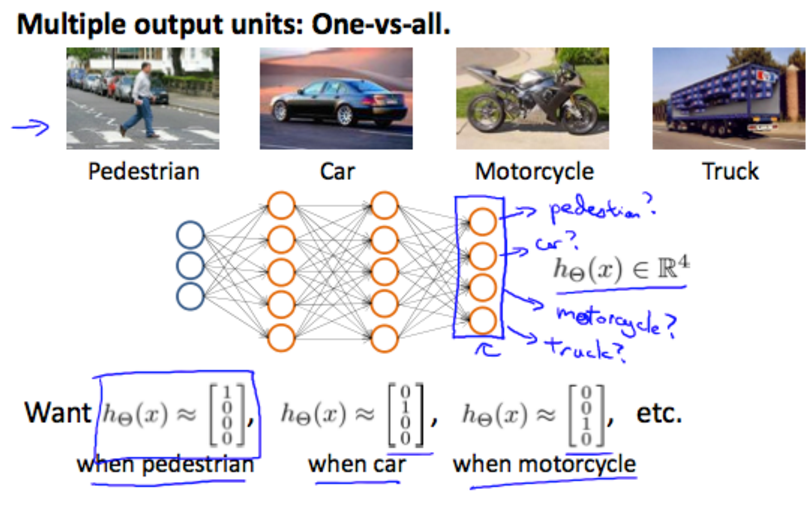
k代表输出单元数/层数
i代表特征数:0-m
j代表网络层数
L代表网络总层数
SL代表网络在第l层的单元数量(sl = number of units (not counting bias unit) in layer l)
Note:
- the double sum simply adds up the logistic regression costs calculated for each cell in the output layer
- the triple sum simply adds up the squares of all the individual Θs in the entire network.
- the i in the triple sum does not refer to training example i
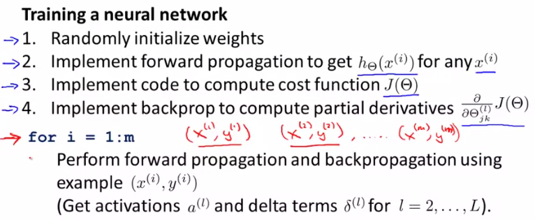
5.3backpropogation
definition: backpropogation is a termonology to minimize the cost function
backpropogation algorithm 反向传播算法
in order to minimize the cost function, then we gradually do this
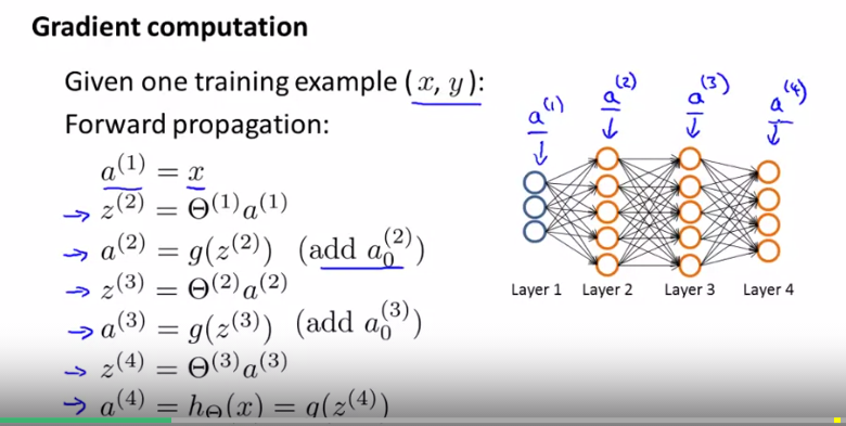
gradient computation
误差值计算
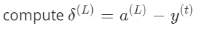

公式

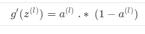
第l层激活函数导数
累加器D
当j=0是,即为biases
当j is not 0,即为the gradient of cost function to the weights

backpropogation的进一步解释,联系权重,对输出值的偏导,概率值等。
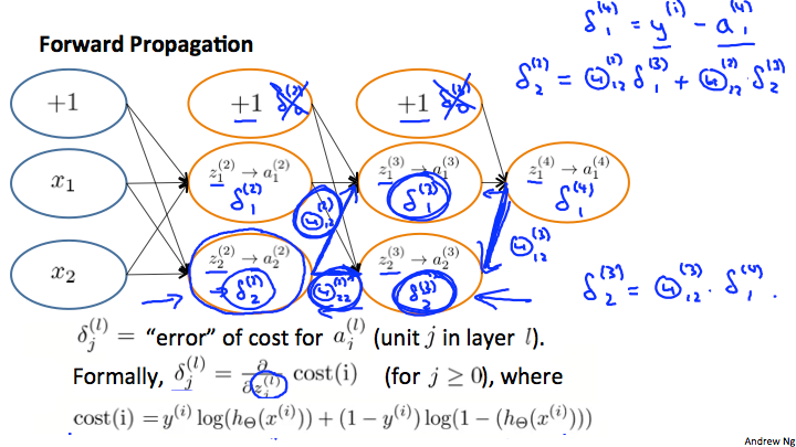
误差=y值-概率值
误差=cost对输出值的偏导,cost=y*log(h)+(1-y)*log(1-h)
5.4backpropogation
In order to use the optimization function, such as fminunc, we should convert the matrix of theta 1-3 to matrix of DVec.
how to convert the matrix of theta to the matrix of Digital D, and reshape the matrix of thetavec

use forward propogation and backword propogation, we can get the data of theta, thetaVec, and J(theta) which is cost function or gradientVec
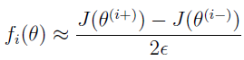
5.5近似计算cost对权值的倒数
计算cost对权值导数可以求得thetaVec,即累加器
对于2个向量和n个向量的方程分别如下,
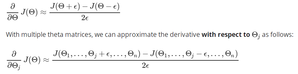
对应于n个向量,在octave中,代码如下,
epsilon = 1e-4;
for i = 1:n,
  thetaPlus = theta;
  thetaPlus(i) += epsilon;
  thetaMinus = theta;
  thetaMinus(i) -= epsilon;
  gradApprox(i) = (J(thetaPlus) - J(thetaMinus))/(2*epsilon)
end;
这样就得到了n次迭代后,累加器值。
5.6神经网络知识点汇总
5.6.1选择网络结构
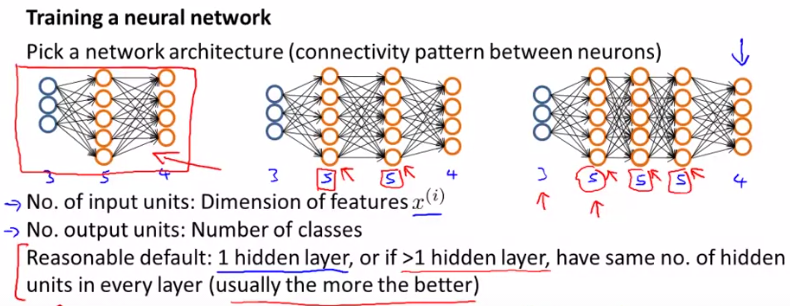
5.6.2训练神经网络

5.7homework
5.7.1visualizing the data for the neural network

5.7.2model representation
load matrix of weights of theta1 and theta2 to compute the a and z
5.7.3feedforward and cost function
zeros(size(theta1)) 设置theta1矩阵所有变量为0
ones(m,1)表示m行1列的全为1的元素,比如ones(8,1)这个表示8行1列全为1的元素
eye()产生mxn的单位矩阵
%m = size(X, 1);
%part1 计算假设函数
a1 = [ones(m,1) X]; %对X添加1列,也可写成 a1 = [ones(size(X,1),1) X]
z2 = a1 * Theta1'; %5000x25
a2 = sigmoid(z2);
a2 = [ones(size(a2,1),1) a2];
z3 = a2 * Theta2';
a3 = sigmoid(z3);
h = a3; %5000x10
%y为mx1,需要改成mx10
%先创建一个mxn的10x10的矩阵,再修改m和n值
y_mn = eye(num_labels);
y = y_mn(y,:);
%计算无正则项的cost function
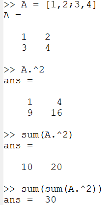
%向量乘向量需要点乘 .*
J = (-1/m) * sum(sum(y.*log(h)+(1-y).*log(1-h)));
计算结果如下:
Feedforward Using Neural Network ...
Cost at parameters (loaded from ex4weights): 0.287629
(this value should be about 0.287629)
5.7.4regularized cost function
什么时候用点乘 " .* ":如果求下来,结果是矩阵,这个时候用点乘;相当于矩阵对应每个元素之间做运算
什么时候用乘 " * ":如果求下来,结果是一个数,这个时候用乘。

两次sum函数之后,结果就是一个数
对于这里的regularized cost function,采用两种做法,第一种直接算,不在theta里面采用向量运算,第二种在theta里面采用向量运算
%方法1
sum1 = 0;
sum2 = 0;
for i = 1 : size(Theta1,1)
  sum1 += Theta1(i,:) * Theta1'(:,i) - sum(Theta1(i,1).^2);
endfor
for j=1:size(Theta2,1)
  sum2 += Theta2(j,:) * Theta2'(:,j) - sum(Theta2(j,1).^2);
endfor
J += lambda/(2*m) * (sum1+sum2);

%方法2
##regularization = lambda/(2*m) * (sum(sum(Theta1(:,2:end).^2)) + sum(sum(Theta2(:,2:end).^2)));
##J +=  regularization;
backpropagation
5.7.5 sigmoid gradient
at first, the sigmoid gradient should be finished.

g = sigmoid(z) .* (1 - sigmoid(z));
so we can get a vector with five sigmoid value
Sigmoid gradient evaluated at [-1 -0.5 0 0.5 1]:
0.196612 0.235004 0.250000 0.235004 0.196612
5.7.6random initialization
设置好初始的epsilon值,代入equation中,得到权值矩阵
epsilon_init = 0.12;
W = rand(L_out, 1 + L_in) * 2 * epsilon_init -  epsilon_init;
5.7.7update backpropagation
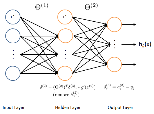
there are five steps to do this part:
1.add one raw to a1 to match the size of Theta1;
2.then to compute the delta3,
![]()
3.continously compute the delta2(hidden layer) according to the delta3(output layer)
![]()
4.starting from 2 of the delta to the end, just skipping the delta0
![]()
5.obtain the unregularized gradient for the neural network cost function by dividing the m which is the examples of tasks

X = [ones(m,1) X] %5000x401
for t = 1:m
  a1 = X(t,:); %1x401
  a1 = a1'; %401x1
  z2 = Theta1 * a1;  %25x1
  a2 = sigmoid(z2);
  a2 = [1 ; a2];  %26X1
  z3 = Theta2 * a2; %10X1
  a3 = sigmoid(z3); %10x1
  h = a3; %10x1

  %y为5000x1,需要改成5000x10
  %先创建一个mxn的10x10的矩阵,再修改m和n值
  y_temp = zeros(num_labels,1); %10x1
  y_temp(y(t)) = 1;
  J += (-1/m) * sum(sum(y_temp.*log(h)+(1-y_temp).*log(1-h)));

%backpropagation
  delta3 = a3 - y_temp; %10x1
  delta2 = Theta2(:,2:end)' * delta3 .* sigmoidGradient(z2); %25x1 x 25x1 =25x1
  Theta1_grad += delta2 * a1'; %25x401
  Theta2_grad += delta3 * a2'; %10x26
endfor

Theta1_grad = Theta1_grad / m;
Theta2_grad = Theta2_grad / m;
5.7.7gradient check
5.7.8regularized neural networks

Theta1(:,1) = 0;
Theta2(:,1) = 0;
Theta1_grad += lambda/m * Theta1;
Theta2_grad += lambda/m * Theta2;
week6 how to optimize a machine learning algorithm
6.1evaluate a learning algorithm
in order to evaluate the algorithm, we split up the data into two sets that are a training set(70%) and a testing set(30%).
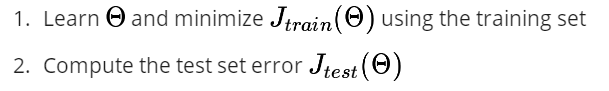
on the process of test, we set error.
for linear regression, it is
![]()
for classification/multiclassification, it is

and the err(h) could be divided into two parts, they are,

6.2model selection and train, validation, test sets
cross validation - CV

6.3the difference for setting high bias and high variance
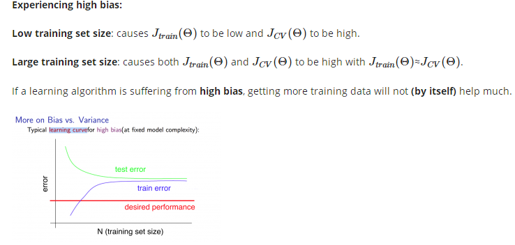
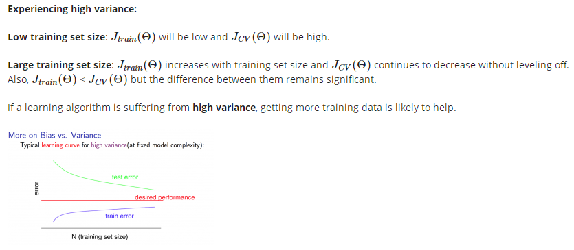
if J_train is much less than J_cv, it is possible that a learning algorithm is suffering from high bias and getting more train data/decreasing the hidden layer which is means to make the model less difficult is unlikely to help much. Additionally, it is possible that a learning algorithm is suffering from high variance and getting more train data/decreasing the hidden layer which is means to make the model less difficult is likely to help.
6.4debugging a learning algorithm
减小算法误差
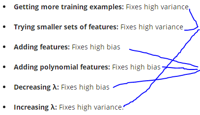
getting more training examples == trying smaller sets of features == a neural network with fewer parameters == increasing lambda are equal to make the neural network less complex to underfit the data/computationally cheaper;
adding features == adding polynomial features == a large neural network with more parameters == decreasing lambda are equal to make the neural network more complex to overfit the data/computationally expensive.
6.5homework
6.5.1linear regression cost function
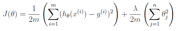
regularization = lambda/(2*m) * sum(theta(2:end).^2);
J = 1/(2*m) * sum((X*theta-y)'*(X*theta-y)) + regularization;
the initialized result is 303.99 and the plotdata is below

6.5.2regularization gradient
in this part, regularization gradient should be finished.
the equation is defined by that

grad = (X'*(X*theta-y))/m;
grad(2:end) = grad(2:end) + lambda*theta(2:end)/m;
and the result is Gradient at theta = [1 ; 1]: [-15.303016; 598.250744]
6.5.3fitting linear regression
visualize the data or in the next section a function can be used to generate learning curves.

6.5.4bias-variance
high bias causes underfit and high variance causes overfit.
using the data as followed to plot the figure from 1 to i
for i = 1:m
  theta = trainLinearReg(X(1:i,:),y(1:i),0);
  error_train(i) = linearRegCostFunction(X(1:i,:),y(1:i),theta,0);
  error_val(i) = linearRegCostFunction(Xval,yval,theta,0);
endfor
6.5.5ploy features
put the multi-features into the X_poly, so we can get a matrix of [m x p] instead of [m x 1]. It can allow us to add more features into the X rather than just one value.
the function maps the original training set X of size mx1 into its higher powers. Speci cally, when a training set X of size mx1 is passed into the function, the function should return a mxp matrix X poly.
where column 1 holds the original values of X, column 2 holds the values of X.^2, column 3 holds the values of X.^3, and so on.
for i=1:p
  X_poly(:,i) = X.^i;
endfor
X(i).^2与X.^2的区别:
X(i).^2表示某一行内积平方;
X.^2表示这个向量内积平方。
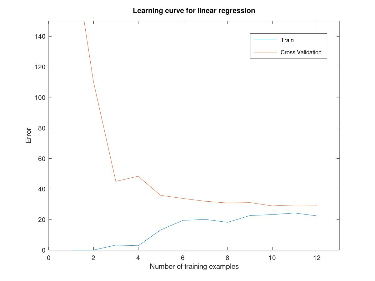
6.5.6learning Polynomial regression
设置完参数后,这里就会出现过拟合现象,因为training error is low, but cross validation is high, so in this case, the model is in a situation of high variance.
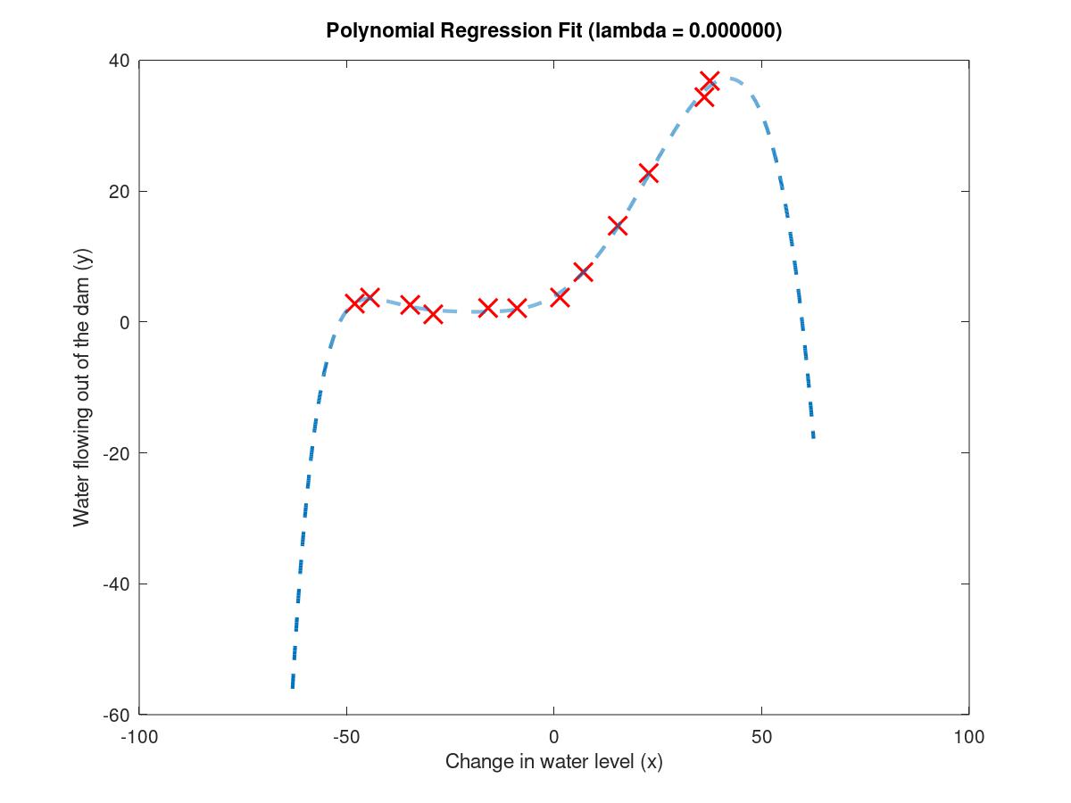
polynomial fit
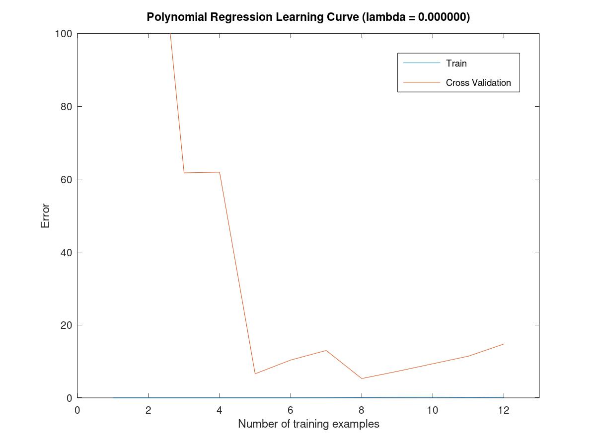
polynomial learning curve
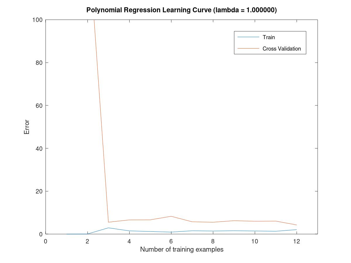
6.5.6adjust the regularization parameter
when the lambda is 1, the data are matched well.

and the cross validation error is obviously decreased.
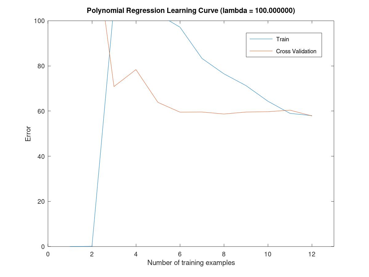
when the lambda is 100, the figure is underfitted and it is situated in the stage of high bias.

6.5.7select a lambda to use a cross validation set
在调用trainLinearReg函数时,不能写成theta = trainLinearReg(X(1:i,:),y(1:i),lambda);
因为这代表在传参数时就部分传入,其实应该在传入时,整体传入,处理时,部份处理写成X(1:i,:), y(1:i);
同时在训练时,对累加数据进行训练,在交叉验证时,对所有数据进行处理。
正则化的使用情况是:对overfitting的figure做处理;所以在计算cost function = train_error/validation_error时,就不用再次正则化,因为需要控制变量。
一方面需要看lambda对曲线的影响,如果加上正则化,就是两个因素影响曲线,所以这里取消正则化,即设置lambda=0
for i = 1:length(lambda_vec)
  lambda = lambda_vec(i);
  theta = trainLinearReg(X,y,lambda);
  error_train(i) = linearRegCostFunction(X,y,theta,0)
  error_val(i) = linearRegCostFunction(Xval,yval,theta,0)
endfor
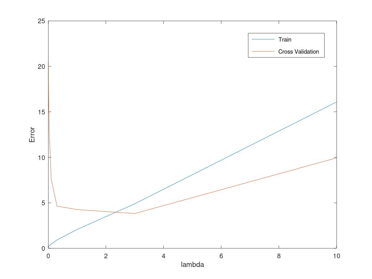 get the parameter of lambda=3 which is the minimun of error of cross validation
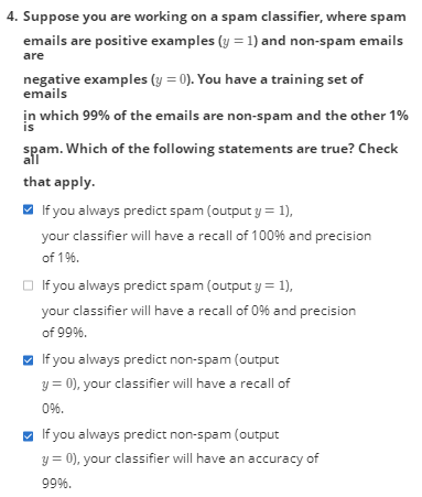
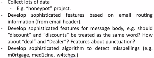
6.6building a spam classifier
6.6.1prioritizing what to work on
the recommended method to solve the ML problem
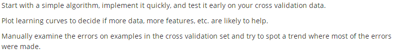
quick and dirty implementation to get the result
then a optimization can be done with a more accurated direction
6.6.2Error Metrics for Skewed Classes
通过precision and recall, 用来优化算法,即使有极限扭曲的现象。
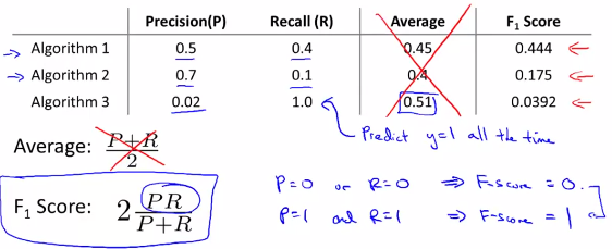
6.6.3Trade off precision and recall
pick up a formula to compute the F score which is equal F = (P*R) / (P+R), instead F = (P + R) / 2
通过F值计算来考察算法的优劣,precision应稍高,recall应略低
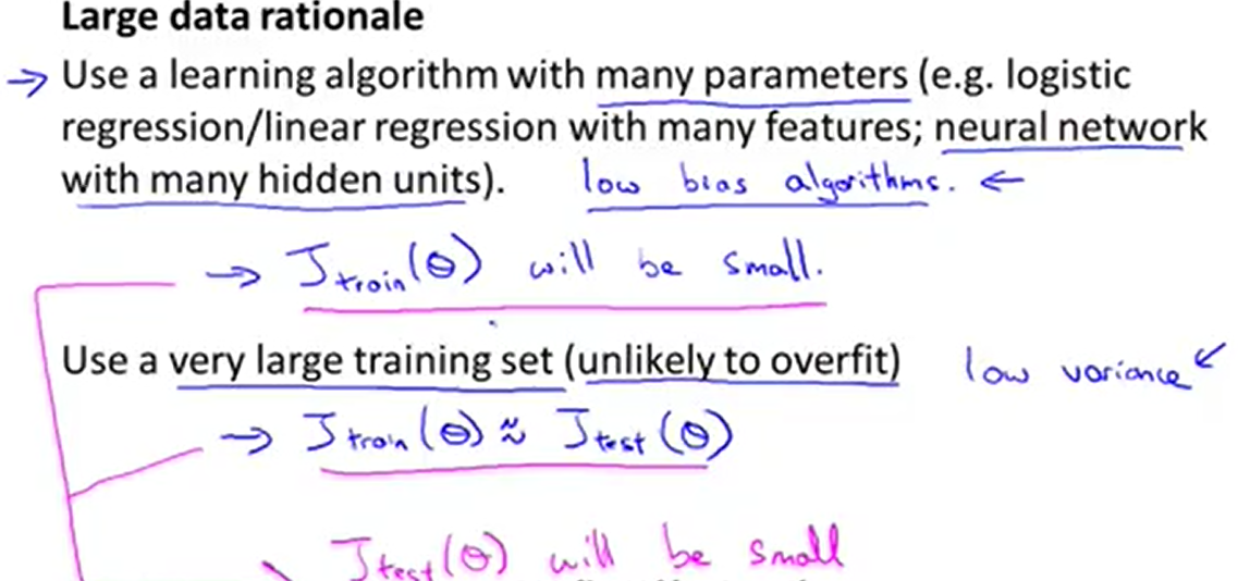
6.7using large data set
design a high accuracy learning system
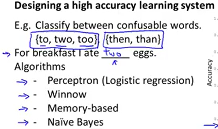
large data rationale, there are three points to optimise
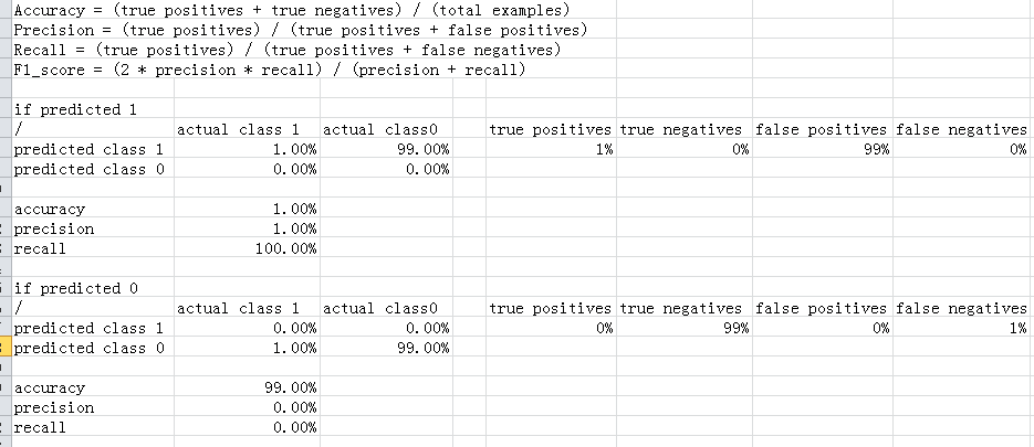
6.8 experiment
关于计算predict 1的accuracy,precision and recall,有练习和公式