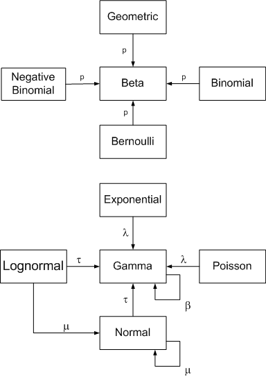
The following diagram summarizes conjugate prior relationships for a number of common sampling distributions.
Arrows point from a sampling distribution to its conjugate prior distribution. The symbol near the arrow indicates which parameter the prior is unknown.
These relationships depends critically on choice of parameterization, some of which are uncommon. This page uses the parameterizations that make the relationships simplest to state, not necessarily the most common parameterizations. See footnotes below.
Click on a distribution to see its parameterization. Click on an arrow to see posterior parameters.
See this page for more diagrams on this site including diagrams for probability and statistics, analysis, topology, and category theory. Also, please contact me if you’re interested in Bayesian statistical consulting.
Parameterizations
Let C(n, k) denote the binomial coefficient(n, k).
The geometric distribution has only one parameter, p, and has PMF f(x) = p (1-p)x.
The binomial distribution with parameters n and p has PMF f(x) = C(n, x) px(1-p)n-x.
The negative binomial distribution with parameters r and p has PMF f(x) = C(r + x – 1, x)pr(1-p)x.
The Bernoulli distribution has probability of success p.
The beta distribution has PDF f(p) = Γ(α + β) pα-1(1-p)β-1 / (Γ(α) Γ(β)).
The exponential distribution parameterized in terms of the rate λ has PDF f(x) = λ exp(-λ x).
The gamma distribution parameterized in terms of the rate has PDF f(x) = βα xα-1exp(-β x) / Γ(α).
The Poisson distribution has one parameter λ and PMF f(x) = exp(-λ) λx/ x!.
The normal distribution parameterized in terms of precision τ (τ = 1/σ2)
has PDF f(x)
= (τ/2π)1/2 exp( -τ(x –
μ)2/2 ).
The lognormal distribution parameterized in terms of precision τ has PDF f(x) = (τ/2π)1/2exp( -τ(log(x) – μ)2/2 ) / x.
Posterior parameters
For each sampling distribution, assume we have data x1, x2, …, xn.
If the sampling distribution for x is binomial(m, p) with m known, and the prior distribution is beta(α, β), the posterior distribution for p is beta(α + Σxi, β + mn – Σxi). The Bernoulli is the special case of the binomial with m = 1.
If the sampling distribution for x is negative binomial(r, p) with r known, and the prior distribution is beta(α, β), the posterior distribution for p is beta(α + nr, β + Σxi). Thegeometric is the special case of the negative binomial with r = 1.
If the sampling distribution for x is gamma(α, β) with α known, and the prior distribution on β is gamma(α0, β0), the posterior distribution for β is gamma(α0 + n, β0 + Σxi). Theexponential is a special case of the gamma with α = 1.
If the sampling distribution for x is Poisson(λ), and the prior distribution on λ is gamma(α0, β0), the posterior on λ is gamma(α0 + Σxi, β0 + n).
If the sampling distribution for x is normal(μ, τ) with τ known, and the prior distribution on μ is normal(μ0, τ0), the posterior distribution on μ is normal((μ0 τ0 + τ Σxi)/(τ0 + nτ), τ0 + nτ).
If the sampling distribution for x is normal(μ, τ) with μ known, and the prior distribution on τ is gamma(α, β), the posterior distribution on τ is gamma(α + n/2, (n-1)S2) where S2 is the sample variance.
If the sampling distribution for x is lognormal(μ, τ) with τ known, and the prior distribution on μ is normal(μ0, τ0), the posterior distribution on μ is normal((μ0 τ0 + τ Πxi)/(τ0 + nτ), τ0 +nτ).
If the sampling distribution for x is lognormal(μ, τ) with μ known, and the prior distribution on τ is gamma(α, β), the posterior distribution on τ is gamma(α + n/2, (n-1)S2) where S2 is the sample variance.
References
A compendium of conjugate priors by Daniel Fink.
See also Wikipedia’s article on conjugate priors.