接着昨天的工作继续。定位的过程有些是基于车牌的颜色进行定位的,自己则根据数字图像一些形态学的方法进行定位的。
合着代码进行相关讲解。
1.相对彩色图像进行灰度化,然后对图像进行开运算。再用小波变换获取图像的三个分量。考虑到车牌的竖直分量较为丰富,选用竖直分量进行后续操作。注意下,这里的一些参数可能和你的图片大小有关,所以要根据实际情况调整。
Image=imread('D:1_2学习图像处理车牌识别matlab_car_plate-recognizationcar_examplecar0.jpg');%获取图片
im=double(rgb2gray(Image));
im=imresize(im,[1024,2048]);%重新设置图片大小  [1024,2048]
% % 灰度拉伸
% % im=imadjust(Image,[0.15 0.9],[]);
  s=strel('disk',10);%strei函数
 Bgray=imopen(im,s);%打开sgray s图像
% % figure,imshow(Bgray);title('背景图像');%输出背景图像
% %用原始图像与背景图像作减法,增强图像
 im=imsubtract(im,Bgray);%两幅图相减
% figure,imshow(mat2gray(im));title('增强黑白图像');%输出黑白图像

[Lo_D,Hi_D]=wfilters('db2','d'); % d Decomposition filters
[C,S]= wavedec2(im,1,Lo_D,Hi_D); %Lo_D  is the decomposition low-pass filter
% decomposition vector C    corresponding bookkeeping matrix S
isize=prod(S(1,:));%元素连乘
%
cA   = C(1:isize);%cA  49152
cH  = C(isize+(1:isize));
cV  = C(2*isize+(1:isize));
cD  = C(3*isize+(1:isize));
%
cA   = reshape(cA,S(1,1),S(1,2));
cH  = reshape(cH,S(2,1),S(2,2));
cV  = reshape(cV,S(2,1),S(2,2));
cD  = reshape(cD,S(2,1),S(2,2));
获取结果
2. 对上面过程中获取的图像进行边沿竖直方向检测,再利用形态学的开闭运算扩大每个竖直方向比较丰富的区域。最后对不符合区域进行筛选。部分代码:
I2=edge(cV,'sobel',thresh,'vertical');%根据所指定的敏感度阈值thresh,在所指定的方向direction上,
a1=imclearborder(I2,8); %8连通 抑制和图像边界相连的亮对象
se=strel('rectangle',[10,20]);%[10,20]
I4=imclose(a1,se);
st=ones(1,8); %选取的结构元素
bg1=imclose(I4,st); %闭运算
bg3=imopen(bg1,st); %开运算
bg2=imopen(bg3,[1 1 1 1]');
I5=bwareaopen(bg2,500);%移除面积小于2000的图案
I5=imclearborder(I5,4); %8连通 抑制和图像边界相连的亮对象
 figure,imshow(I5);title('从对象中移除小对象');
获取的筛选结果:
我们接下来目的就是从这些待选区域中挑选出车牌区域。
3 这里我们就要利用一些关于车牌的先验知识。2007 年实施的车牌标准规定,车前车牌长440mm,宽140mm。其比例为440 /140 ≈3.15 。根据图像像素的大小,这里选取筛选条件为宽在70到250之间,高在15到70之间,同时宽高比例应大于0.45,就可以比较准确的得到车牌的大致位置。当然,这里宽高值也是根据你的图像大小进行设置的,大小不一样,值略有区别。
%利用长宽比进行区域筛选
[L,num] = bwlabel(I5,8);%标注二进制图像中已连接的部分,c3是形态学处理后的图像
Feastats =regionprops(L,'basic');%计算图像区域的特征尺寸
Area=[Feastats.Area];%区域面积
BoundingBox=[Feastats.BoundingBox];%[x y width height]车牌的框架大小
RGB = label2rgb(L,'spring','k','shuffle'); %标志图像向RGB图像转换

lx=1;%统计宽和高满足要求的可能的车牌区域个数
Getok=zeros(1,10);%统计满足要求个数
for l=1:num  %num是彩色标记区域个数
width=BoundingBox((l-1)*4+3);
hight=BoundingBox((l-1)*4+4);
rato=width/hight;%计算车牌长宽比
%利用已知的宽高和车牌大致位置进行确定。
if(width>70 & width<250 & hight>15 & hight<70 &(rato>3&rato<8)&((width*hight)>Area(l)/2))%width>50 & width<1500 & hight>15 & hight<600
        Getok(lx)=l;
        lx=lx+1;
end
end
startrow=1;startcol=1;
[original_hihgt original_width]=size(cA);
当然,这个只是初步确定,经常出现的结果是好几个待选区域都满足要求。通过观察它的直方图发现车牌区域的直方图多波峰波谷,变化大,而一般的区域变化较不明显。因此根据它的方差,波峰波谷值数量来确定车牌区域。实验结果表明效果还是挺不错的。
for order_num=1:lx-1 %利用垂直投影计算峰值个数来确定区域
  area_num=Getok(order_num);
  startcol=round(BoundingBox((area_num-1)*4+1)-2);%开始列
  startrow=round(BoundingBox((area_num-1)*4+2)-2);%开始行
  width=BoundingBox((area_num-1)*4+3)+2;%车牌宽
  hight=BoundingBox((area_num-1)*4+4)+2;%车牌高
  uncertaincy_area=cA(startrow:startrow+hight,startcol:startcol+width-1); %获取可能车牌区域
  image_binary=binaryzation(uncertaincy_area);%图像二值化
  histcol_unsure=sum(uncertaincy_area);%计算垂直投影
   histcol_unsure=smooth(histcol_unsure)';%平滑滤波
      histcol_unsure=smooth(histcol_unsure)';%平滑滤波
      average_vertical=mean(histcol_unsure);
  figure,subplot(2,1,1),bar(histcol_unsure);
  subplot(2,1,2),imshow(mat2gray(uncertaincy_area));
  [data_1 data_2]=size(histcol_unsure);
  peak_number=0; %判断峰值个数
  for j=2:data_2-1%判断峰值个数
      if (histcol_unsure(j)>histcol_unsure(j-1))&(histcol_unsure(j)>histcol_unsure(j+1))
          peak_number=peak_number+1;
      end
  end
   valley_number=0; %判断波谷个数
  for j=2:data_2-1
      if (histcol_unsure(j)<histcol_unsure(j-1))&(histcol_unsure(j)<histcol_unsure(j+1)) &(histcol_unsure(j)<average_vertical)
           %波谷值比平均值小
          valley_number=valley_number+1;
      end
  end
  %peak_number<=15
 if peak_number>=7 & peak_number<=18 &valley_number>=4 & (startcol+width/2)>=original_width/6 &(startcol+width/2)<=5*original_width/6....
     &(startrow+hight/2)>=original_hihgt/6 & (startrow+hight/2)<=original_hihgt*5/6
     %进一步确认可能区域
     select_unsure_area(count)=area_num;
     standard_deviation(count)=std2(histcol_unsure);%计算标准差
     count=count+1;
 end
end
correct_num_area=0;
max_standard_deviation=0;
if(count<=2) %仅有一个区域

    correct_num_area=select_unsure_area(count-1);
else
    for  num=1:count-1
       if(standard_deviation(num)>max_standard_deviation)
           max_standard_deviation=standard_deviation(num);
         correct_num_area=select_unsure_area(num);
       end
    end
end
获取区域: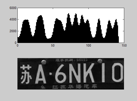
定位大概就这么多。这里说明一下,上面一些参数和你的图片规格有关系,不是你随便拿来一张就可以识别的,要根据你的实际进行调整。大概就这么多,欢迎交流,转载请注明出处,谢谢。