Stat2.3x Inference(统计推断)课程由加州大学伯克利分校(University of California, Berkeley)于2014年在edX平台讲授。
ADDITIONAL PRACTICE FOR THE FINAL
In the following problems you will be asked to choose one of the four options (A)-(D). The options are stated here once and for all. If you pick any option other than (A), you must fill in all blanks correctly for credit. Use the 5% cutoff for P.
(A) The question cannot be answered based on the information given.
(B) one-sample $z$ = ( ); P approx ( ); Conclusion: ( ).
(C) two-sample $z$ = ( ); P approx ( ); Conclusion: ( ).
(D) one-sample $t$ = ( ); d.f. = ( ); P approx ( ); Conclusion: ( ).
PROBLEM 1
A die is rolled 600 times. The face with six spots comes up 126 times. Does the die land "six" with chance 1/6? Or are there too many sixes? Answer the question in the following steps:
a) State the null hypothesis.
b) State the alternative hypothesis.
c) Under the null hypothesis, the number of sixes in the 600 rolls is expected to be ( ), give or take ( ).
d) In this context, pick one of the options (A)-(D).
Solution
a) Null $H_0: p = frac{1}{6}$
b) Alternative $H_A: p >frac{1}{6}$
c) $$E=ncdot p=600 imesfrac{1}{6}=100$$ $$sigma=sqrt{pcdot(1-p)cdot n}=sqrt{frac{1}{6} imesfrac{5}{6} imes600}=9.128709$$
d) This is one-sample $z$ test, (B) is correct. $$z=frac{126-100}{sigma}$$ and P-value is 0.002198659 which is smaller than 0.05, so we reject $H_0$. Thus the conclusion is $p > frac{1}{6}$. R code:
sigma = sqrt(1/6 * 5/6 * 600)
z = (126 - 100) / sigma
1 - pnorm(z)
[1] 0.002198659
PROBLEM 2
A simple random sample of 6 students is taken from among all students in a university. The average age of the sampled students is 20 years with an SD of 3 years. Someone wants to test the hypothesis that the average age of students in the university is 21 years.
a) State the null and alternative hypotheses.
b) If possible, perform a test. [Pick one of the options (A)-(D).]
Solution
a) $$H_0: mu=21$$ $$H_A: mu < 21$$
b) The sample is too small (only 6), the population distribution may be quite far away from normal. So none of our tests apply. (A) is correct.
PROBLEM 3
Five hundred eight-year-olds are participating in a study about the effect of using calculators in math class. Three hundred are chosen at random and allowed to use calculators; the remaining two hundred are not allowed calculators. At the end of the study, 180 of the "calculator" group pass the study's math test, and 150 of the "non-calculator" group pass the same test. Did the calculators have any effect?
a) State null and alternative hypotheses (carefully!).
b) If possible, perform a test. [Pick one of the options (A)-(D).]
Solution
a) $$H_0: p_1 = p_2$$ $$H_A: p_1 < p_2$$ where $p_1, p_2$ represents the percents of passing math test in calculator and non-calculator group, respectively.
b) This is two-sample $z$ test. Since the two samples are from the same population, so we don't use pooled estimate. $$n_1=300, n_2=200, p_1=frac{180}{300}, p_2=frac{150}{200}$$ And under the null we, have $$sigma_{p_1-p_2}=sqrt{sigma_1^2+sigma_2^2} = sqrt{frac{p_1cdot(1-p_1)}{n_1}+frac{p_2cdot(1-p_2)}{n_2}}$$ Thus $$z=frac{p_1-p_2}{sigma_{p_1-p_2}}$$ The P-value is 0.0002614627 which is very tiny. We reject $H_0$, that is, the conclusion is $p_1 < p_2$. R code:
n1 = 300; n2 = 200; p1 = 180/300; p2 = 150/200
sigma1 = sqrt(p1 * (1 - p1) / n1); sigma2 = sqrt(p2 * (1 - p2) / n2)
sigma = sqrt(sigma1^2 + sigma2^2)
z = (p1 - p2) / sigma; pnorm(z)
[1] 0.0002614627
PROBLEM 4
In a simple random sample of 400 eight-year-olds taken in 1990, 15% owned computer games. In an independent simple random sample of 600 eight-year-olds taken in 2000, 35% owned computer games. Was the percent of eight-year-olds who owned computer games higher in 2000 than in 1990? Or is this just chance variation? Answer in the following steps:
a) State a null hypothesis.
b) State an alternative hypothesis.
c) In this context, pick one of the options (A)-(D).
Solution
a) Null $H_0: p_1 = p_2$
b) Alternative $H_A: p_1 < p_2$
c) This is two-sample $z$ test. (C) is correct. The two samples are from two independent populations, so we use pooled estimate. $$n_1=400, n_2=600, p_1=0.15, p_2=0.35$$ And we have $$hat{p}=frac{n_1cdot p_1+n_2cdot p_2}{n_1+n_2}, sigma=sqrt{hat{p}cdot(1-hat{p})cdot(frac{1}{n_1}+frac{1}{n_2})}$$ So $$z=frac{p_1-p_2}{sigma}$$ The P-value is $1.486594 imes10^{-12}$ which is close to zero. Thus we reject $H_0$ and conclude that $p_1 < p_2$. R code:
n1 = 400; n2 = 600; p1 = 0.15; p2 = 0.35
p = (n1 * p1 + n2 * p2) / (n1 + n2)
sigma = sqrt(p * (1 - p) / n1 + p * (1 - p) / n2)
z = (p1 - p2) / sigma; pnorm(z)
[1] 1.486594e-12
PROBLEM 5
A forest contains large numbers of trees of one species. The distribution of the heights of these trees is normal. A simple random sample of 7 of these trees is taken and their heights measured. The average of these 7 heights is 32 feet and their SD (computed as the ordinary SD of a list, with 7 in the denominator) is 2 feet. In order to test the hypothesis that the average height of all the trees of this species in the forest is 35 feet, follow the steps below.
a) State null and alternative hypotheses clearly.
b) If possible, perform a test. [Pick one of the options (A)-(D).]
Solution
a) $$H_0: mu=35$$ $$H_A: mu < 35$$
b) This is classic $t$ test, that is, the population is normal and the sample is small with unknown population mean (need to be tested) and SD. (D) is correct. Note that this problem is different from Problem 2 whose population may not be normal. We have $$sigma=2 imessqrt{frac{7}{6}}, SE=frac{sigma}{7}, t=frac{32-35}{SE}$$ The P-value is 0.00520086 which is smaller than 0.05, so we reject $H_0$ and conclude that $mu < 35$. R code:
n = 7; sd = 2; mu = 32
se = sd * sqrt(n / (n - 1)) / sqrt(n)
t = (mu - 35) / se; pt(t, 6)
[1] 0.00520086
PROBLEM 6
In 1997, the average MSAT score in a certain state was 430 with an SD of 100. In 1998, a simple random sample of 400 SAT candidates in this state had an average MSAT score of 425 with an SD of 110. In 1999, a simple random sample of 200 SAT candidates in this state had an average MSAT score of 420 with an SD of 105. These students had an average VSAT score of 435 with an SD of 100. In each of parts a), b) and c) below, say whether the question makes sense; then pick one of the options (A)-(D).
a) Is the difference between 430 and 425 statistically significant?
b) Is the difference between 425 and 420 statistically significant?
c) Is the difference between 420 and 435 statistically significant?
Solution
a) This is one-sample $z$ test, (B) is correct. $$H_0: mu=430$$ $$H_A: mu < 430$$ And we have $$n=400, mu=425, sigma=110$$ So $$SE=frac{sigma}{n}, z=frac{425-430}{SE}$$ The P-value is 0.1816511 which is larger than 0.05, so we reject $H_A$ and conclude that $mu = 430$. R code:
n = 400; sigma = 110
se = sigma / sqrt(n)
z = (425 - 430) / se
pnorm(z)
[1] 0.1816511
b) There are two independent simple random samples, so this is two-sample $z$ test. (C) is correct. $$H_0: mu_1=mu_2$$ $$H_A: mu_1 > mu_2$$ We have $$mu_1=425, mu_2=420, sigma_1=110, sigma_2=105, n_1=400, n_2=200$$ And $$SE=sqrt{SE_1^2+SE_2^2}=sqrt{frac{sigma_1^2}{n_1}+frac{sigma_2^2}{n_2}}, z=frac{mu_1-mu_2}{SE}$$ The P-value is 0.2942077 which is larger than 0.05, so we reject $H_A$ and conclude that $mu_1=mu_2$. R code:
n = 400; sigma = 110
se = sigma / sqrt(n)
z = (425 - 430) / se
pnorm(z)
[1] 0.1816511
PROBLEM 7
A factory produces widgets that are supposed to weigh 50 mg. The histogram of weights follows the normal curve with an SD of 5 mg. In a simple random sample of 9 of the widgets, the average weight is 52 mg with an SD of 3 mg (computed as the ordinary SD of a list, with 9 in the denominator). On average, are the widgets produced by the factory heavier than 50 mg? Or is this chance variation? Answer in the following steps.
a) State the null hypothesis.
b) State the alternative hypothesis.
c) In this context, pick one of the options (A)-(D).
Solution
a) Null $$H_0: mu=50$$
b) Alternative $$H_A: mu > 50$$
c) Although the sample size is only 9, this is not a $t$ test since its population SD is known. So this is one-sample $z$ test. (B) is correct. We have $$n=9, mu=52, sigma=5$$ Note that the sample SD is not needed since we know the population SD. Thus $$SE = frac{sigma}{sqrt{n}}, z=frac{52-50}{SE}$$ The P-value is 0.1150697 which is larger than 0.05, so we reject $H_A$ and conclude that $mu=50$. R code:
n = 9; sigma = 5; mu = 52
se = sigma / sqrt(n)
z = (mu - 50) / se
1 - pnorm(z)
[1] 0.1150697
PROBLEM 8
A simple random sample of 200 students is taken at a large university. In the sample, 40% of the students own an iPod and 45% own a laptop computer. At the university, is the percent of students who own a laptop higher than the percent who own an iPod? Or is this just chance variation? Answer in the following steps:
a) State null and alternative hypotheses (carefully!).
b) If possible, perform a test. [Pick one of the options (A)-(D).]
Solution
a) $$H_0: p_1=p_2$$ $$H_A: p_1 < p_2 $$ where $p_1, p_2$ represents the percents of iPod and laptop, respectively.
b) The samples are paired and there is no measure of dependency between the pairs, so (A) is correct.
FINAL EXAM
If a problem asks for an approximation, please use the methods described in the video lecture segments. Unless the problem says otherwise, please give answers correct to one decimal place according to those methods. Some of the problems below are about simple random samples. If the population size is not given, you can assume that the correction factor for standard errors is close enough to 1 that it does not need to be computed. Please check units of measurements in the answers, so that you don't run into trouble with autograding. If you are asked to provide the answer as a percent, and your answer is 90%, please enter 90 but not 90%, nor 0.9, nor 9/10, etc. Please use the 5% cutoff for P-values unless otherwise instructed in the problem.
PROBLEM 1
A statistician analyzing a randomized controlled experiment has tested the following hypotheses: Null: The treatment does nothing. Alternative: The treatment does something. using a 4% cutoff for P-values. The P-value of the test turns out to be about 1.8%. Based on this information, solve Problems 1A-1B.
1A The conclusion of the test is The treatment does nothing. The treatment does something.
1B "$P=1.8%$ means that there is only about a 1.8% chance that the treatment does nothing." The quoted statement is True False
Solution
1A) $1.8\% < 4\%$ so reject $H_0$, that is, the conclusion is "the treatment does something".
1B) False. $P=1.8\%$ means that if the treatment did nothing, there would be about a 1.8% chance of seeing the data in the experiment or data that looked even more as though the treatment does something.
PROBLEM 2
A coin will be tossed 15 times, and I have to decide whether it lands heads with chance 0.6 or 0.3. I'll test the hypotheses Null: $p = 0.6$ Alternative: $p = 0.3$ Based on this information, solve Problems 2A-2C.
2A First, I will use a simple decision rule: if fewer than half the tosses are heads, I will choose $p=0.3$; if more than half the tosses are heads, I will choose $p=0.6$. The significance level of this test is ( )%.
2B The power of the test in Problem 2A is ( )%.
2C Suppose I want to create a new decision rule that says, "If the number of heads is less than H, then I will choose $p=0.3$; otherwise I will choose $p=0.6$." Here H is an integer in the range 0 through 15. Is it possible for me to choose H so that the new test has a smaller significance level as well as a higher power than the test in Problem 2A? Maybe, there is not enough information to decide. Yes. No.
Solution
2A) Significance level is under $H_0$ but concludes $H_A$. By binomial distribution, $$sum_{k=0}^{7}C_{15}^{k}cdot0.6^kcdot(1-0.6)^{15-k}=21.31032\%$$ R code:
sum(dbinom(0:7, 15, 0.6))
[1] 0.2131032
2B) Power is under $H_A$ and concludes $H_A$. By binomial distribution, $$sum_{k=0}^{7}C_{15}^{k}cdot0.3^kcdot(1-0.3)^{15-k}=94.99875\%$$ R code:
sum(dbinom(0:7, 15, 0.3))
[1] 0.9499875
2C) Maximize the power for a given significance level. The following R code shows both of them increasing as H becoming larger. The answer is "No".
siglev = power = NULL
for(k in 0:15){
  siglev = c(siglev, sum(dbinom(0:k, 15, 0.6)))
  power = c(power, sum(dbinom(0:k, 15, 0.3)))
}
plot(0:15, siglev, 'l'); lines(0:15, power)
PROBLEM 3
In a simple random sample of 400 households taken in a large city, 57% of the households contain exactly two people in them; these are called "two-person" households. Construct an approximate 85% confidence interval for the percent of two-person households in the city, and provide the endpoints of the intervals in Problems 3A and 3B. Problem 3C continues the analysis of this sample. Please enter your answers as percents as explained in the introduction to the exam; for example, if your answer is 90%, please enter 90 but not 90%, nor 0.9, nor 9/10, etc.
3A The left endpoint of the interval is about ( )%.
3B The right endpoint of the interval is about ( )%.
3C Another statistician uses the same sample to construct a confidence interval for the percent of two-person households in the city. The interval goes from 52.5% to 61.5%. The confidence level of this interval is about ( )%.
Solution
3A) and 3B) $$hat{p}=0.57, SE=sqrt{frac{hat{p}cdot(1-hat{p})}{n}}$$ And the 85% confidence interval is $$hat{p}pm zcdot SE=[0.5343661, 0.6056339]$$ R code:
p = 0.57; n = 400; se = sqrt(p * (1 - p) / n)
z = qnorm((1 - 0.85) / 2)
p + z * se
[1] 0.5343661
p - z * se
[1] 0.6056339
3C) $$z=frac{61.5\%-52.5\%}{2cdot SE}$$ Thus the confidence level is 93.09211%. R code:
z = (0.615 - 0.525) / (2 * se)
1 - (1 - pnorm(z)) * 2
[1] 0.9309211
PROBLEM 4
In a population of over 15,000 patients, the distribution of systolic blood pressure follows the normal curve. Investigators believe the average systolic blood pressure in the population is 120 mm. The investigators take a simple random sample of 6 patients from this population. The systolic blood pressure measurements of these patients have an average of 113.5 mm and an SD (computed with 6 in the denominator) of 12.2 mm. Is the average systolic blood pressure in the population lower than the investigators think? Or is this just chance variation? Answer following the steps in Problems 4A-4E.
4A The null hypothesis is: The average blood pressure in the population is 120 mm. The average blood pressure in the population is less than 120 mm. The average blood pressure in the population is not equal to 120 mm.
4B The approximate distribution of the appropriate test statistic is (pick the best option) binomial hypergeometric normal t chi-square
4C The test is one-tailed two-tailed
4D The P-value of the test is approximately ( )%
4E "The test supports what the investigators think." The quoted statement is True False
Solution
4A) $$H_0: mu=120$$ $$H_A: mu < 120$$ That is, the null is "the average of the sample is different due to chance."
4B) Population distribution normal; unknown SD; small sample; test is about the population mean. This is the classic setting for the $t$ test.
4C) One-tailed.
4D) $$n=6, mu=113.5, SD=12.2$$ $$Rightarrow sigma=SDcdotsqrt{frac{n}{n-1}}, SE=frac{sigma}{n}, t=frac{mu-120}{SE}$$ The P-value is 14.34901%. R code:
n = 6; mu = 113.5; sd = 12.2
sigma = sd * sqrt(n / (n - 1))
se = sigma / sqrt(n)
t = (mu - 120) / se
pt(t, 5)
[1] 0.1434901
4E) Since P is larger than cutoff (0.05) so we reject $H_A$ and conclude that $mu=120$. The answer is "True".
PROBLEM 5
A simple random sample of 1000 freshmen is taken from among freshmen at all private universities in a state. On average, the sampled freshmen worked for 9.2 hours in the week before the survey, with an SD of 9.9 hours. [Here "worked" means "worked for pay".] Based on this information, solve Problems 5A-5C.
5A The interval "8.6 hours to 9.8 hours" is an approximate 95% confidence interval for the average number of hours worked in the week before the survey by freshmen a. in the sample. b. at all private universities in the state.
5B In the week before the survey, about 2.5% of the freshmen in the sample worked more than ( ) hours. Pick the best option. 29 9.8 NA (that is, unknown based on the given information)
5C Because the sample size is large, the Central Limit Theorem says that the ( ) is roughly normal. Fill in the blank with the best option. a. histogram of hours worked in the week before the survey by the sampled freshmen b. histogram of hours worked in the week before the survey by freshmen at all private universities in the state c. probability histogram of the average number of hours worked in the week before the survey by a simple random sample of 1000 freshmen taken from private universities in the state d. probability histogram of the average number of hours worked in the week before the survey by freshmen at all private universities in the state
Solution
5A) The average number of hours worked by the freshmen in the sample is known to be 9.2 hours. The confidence interval estimates the unknown parameter in the population. (b) is correct. We can calculate it as follows: $$mu=9.2, sigma=9.9, n=1000$$ $$Rightarrow SE=frac{sigma}{sqrt{n}}$$ The 95% confidence interval is $$mupm zcdot SE=[8.586403, 9.813597]$$ R code:
n = 1000; sigma = 9.9; mu = 9.2
se = sigma / sqrt(n)
z = qnorm((1 - 0.95) / 2)
mu + z * se
[1] 8.586403
mu - z * se
[1] 9.813597
5B) The distribution of the sampled hours is clearly non-normal ($9.2-9.9 < 0$ which is only 1 unit SD from the mean), and there is not enough information about its shape to fill in the blank. So choose "NA".
5C) The CLT is about probability histograms of sums (and hence averages) of large samples drawn at random. (c) is correct.
PROBLEM 6
A statistician believes that in her town each child born has a 50% chance of being a girl, independently of all other children. There are 281 three-child families in her town; 39 of these families have no girls, 94 have one girl, 115 have two girls, and the remaining 33 have three girls. Say whether the data support the statistician's belief, by following the steps in Problems 6A-6F.
6A If the statistician's belief is correct, the probability that a three-child family in the town will have exactly one girl is ( )%.
6B If the statistician's belief is correct, then among the three-child families in the town what is the expected number of families that have exactly one girl?
6C If the statistician's belief is correct, then among the three-child families in the town what is the expected number of families that have no girls?
6D To test whether the data support the statistician's belief, the appropriate test statistic roughly follows a ( ) distribution. normal t chi-square
6E The P-value of the appropriate test is about ( )%.
6F The conclusion of the test is that the data support the statistician's belief. do not support the statistician's belief.
Solution
6A) Binomial distribution, $$C_{3}^{1} imes0.5 imes0.5^2=37.5\%$$
6B) $$E( ext{one girl})=ncdot p=281 imes0.375=105.375$$
6C) $$E( ext{zero girl})=ncdot p=281 imes C_{3}^{0} imes0.5^0 imes0.5^3=281 imes0.125=35.125$$
6D) chi-square test for categorical data.
6E) $$H_0: ext{the model is good}$$ $$H_A: ext{the model is not good}$$ By binomial distribution, $$E( ext{two girls})=281 imes C_{3}^{2} imes0.5^2 imes0.5=105.375$$ $$E( ext{three girls})=281 imes C_{3}^{3} imes0.5^3=35.125$$ Using the following table:
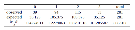
So $chi^2=2.663108$ and the degree of freedom is $4-1=3$. The P-value is 0.4465332. R code:
o = c(39, 94, 115, 33)
e = c(35.125, 105.375, 105.375, 35.125)
chi = sum((o - e)^2 / e); chi
[1] 2.663108
1 - pchisq(chi, 3)
[1] 0.4465332
6F) Because the P-value is large, we reject $H_A$ and conclude that the data support the statistician's belief.
PROBLEM 7
One year, a simple random sample of 1,000 U.S. 10-year-olds was taken. The children were studied for the entire year. At the beginning of the year the sampled children had an average weight of 70 pounds with an SD of 15 pounds. At the end of the year their weights averaged 75 pounds and the SD was 14.5 pounds. The correlation between their weights at beginning and end of the year was 0.8. Based on this information, solve Problems 7A-7B.
7A An approximate 90% confidence interval for the year-end weight of U.S. 10-year-olds that year is 75 pounds plus or minus about ( ) pounds. Fill in the blank with the best of the options below. NA (this blank cannot be filled in with the information given) 0.45 0.75 0.9 24 28
7B Define the weight gain of a child to be "end of year weight - beginning of year weight". The gain is negative if the child weighs less at the end of the year than at the beginning. An approximate 95% confidence interval for the average weight gain of U.S. 10-year-olds that year is 5 pounds plus or minus about ( ) pounds. Fill in the blank with the best of the options below. NA (this blank cannot be filled in with the information given) 0.15 0.3 0.6 9 18 21
Solution
7A) $$n=1000, sigma=14.5, mu=75$$ $$Rightarrow SE=frac{sigma}{sqrt{n}}$$ 90% confidence interval $$z cdot SE=0.7542152$$ R code:
n = 1000; sigma = 14.5
se = sigma / sqrt(n)
z = qnorm((1 - 0.9) / 2)
z * se
[1] -0.7542152
7B) This is paired variables sample. $$sigma_1=14.5, sigma_2=15, n=1000, r=0.8$$ $$Rightarrow sigma_{ ext{difference}}=sqrt{sigma_1^2 + sigma_2^2-2cdotsigma_1cdotsigma_2}, SE=frac{sigma_{ ext{difference}}}{sqrt{n}}$$ And 95% confidence interval is $$zcdot SE=0.5789363$$ R code:
n = 1000; sigma1 = 14.5; sigma2 = 15; r = 0.8
sigma = sqrt(sigma1^2 + sigma2^2 - 2 * r * sigma1 * sigma2)
se = sigma / sqrt(n)
z = qnorm((1 - 0.95) / 2)
z * se
[1] -0.5789363