一.数据产生
 1 from sklearn.datasets import make_classification, make_blobs
 2 from matplotlib.colors import ListedColormap
 3 from sklearn.datasets import load_breast_cancer
 4 from adspy_shared_utilities import load_crime_dataset
 5
 6 cmap_bold = ListedColormap(['#FFFF00', '#00FF00', '#0000FF','#000000'])
 7
 8 #make_regression:随机产生回归模型的数据
 9 #参数:n_samples : 数据个数
10 #n_features:数据中变量个数
11 #n_informative:有关变量个数
12 #bias:线性模型中的偏差项
13 #noise:高斯分布的标准差
14 #random_state:随机数的种子生成器
15
16 # 简单(一个参数)的回归数据
17 from sklearn.datasets import make_regression
18 plt.figure()
19 plt.title('Sample regression problem with one input variable')
20 X_R1, y_R1 = make_regression(n_samples = 100, n_features=1,
21                             n_informative=1, bias = 150.0,
22                             noise = 30, random_state=0)
23 plt.scatter(X_R1, y_R1, marker= 'o', s=50)
24 plt.show()
25
26
27 # 复杂(多参)的回归数据产生
28 from sklearn.datasets import make_friedman1
29 plt.figure()
30 plt.title('Complex regression problem with one input variable')
31 X_F1, y_F1 = make_friedman1(n_samples = 100,
32                            n_features = 7, random_state=0)
33
34 plt.scatter(X_F1[:, 2], y_F1, marker= 'o', s=50)
35 plt.show()
36
37 # 分类模型的数据生成
38 plt.figure()
39 plt.title('Sample binary classification problem with two informative features')
40 X_C2, y_C2 = make_classification(n_samples = 100, n_features=2,
41                                 n_redundant=0, n_informative=2,
42                                 n_clusters_per_class=1, flip_y = 0.1,
43                                 class_sep = 0.5, random_state=0)
44 plt.scatter(X_C2[:, 0], X_C2[:, 1], c=y_C2,
45            marker= 'o', s=50, cmap=cmap_bold)
46 plt.show()
47
48
49 # more difficult synthetic dataset for classification (binary)
50 # with classes that are not linearly separable
51 X_D2, y_D2 = make_blobs(n_samples = 100, n_features = 2, centers = 8,
52                        cluster_std = 1.3, random_state = 4)
53 y_D2 = y_D2 % 2
54 plt.figure()
55 plt.title('Sample binary classification problem with non-linearly separable classes')
56 plt.scatter(X_D2[:,0], X_D2[:,1], c=y_D2,
57            marker= 'o', s=50, cmap=cmap_bold)
58 plt.show()
59
60
61 # 乳腺癌分类数据集
62 cancer = load_breast_cancer()
63 (X_cancer, y_cancer) = load_breast_cancer(return_X_y = True)
64
65
66 # Communities and Crime dataset
67 (X_crime, y_crime) = load_crime_dataset()


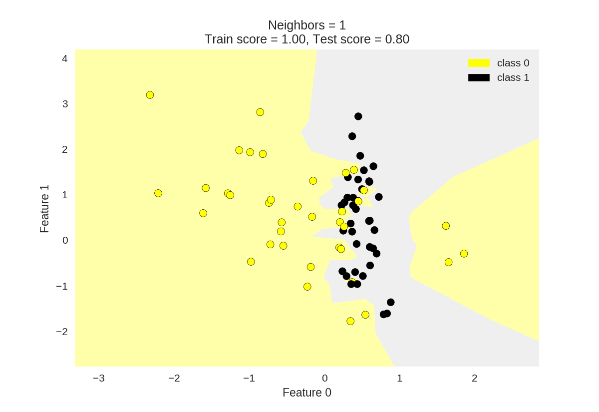
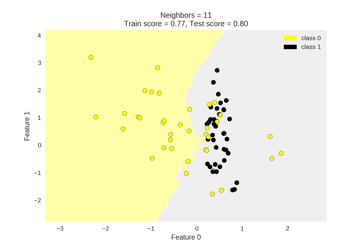
KNN分类
1 from adspy_shared_utilities import plot_two_class_knn
2
3 X_train, X_test, y_train, y_test = train_test_split(X_C2, y_C2,
4                                                    random_state=0)
5
6 #k为knn所选最近邻居个数
7 plot_two_class_knn(X_train, y_train, 1, 'uniform', X_test, y_test)
8 plot_two_class_knn(X_train, y_train, 3, 'uniform', X_test, y_test)
9 plot_two_class_knn(X_train, y_train, 11, 'uniform', X_test, y_test)

KNN回归预测
1 from sklearn.neighbors import KNeighborsRegressor
2
3 X_train, X_test, y_train, y_test = train_test_split(X_R1, y_R1, random_state = 0)
4
5 knnreg = KNeighborsRegressor(n_neighbors = 5).fit(X_train, y_train)
6
7 print(knnreg.predict(X_test))
8 print('R-squared test score: {:.3f}'
9      .format(knnreg.score(X_test, y_test)))
[ 231.71  148.36  150.59  150.59   72.15  166.51  141.91  235.57  208.26
  102.1   191.32  134.5   228.32  148.36  159.17  113.47  144.04  199.23
  143.19  166.51  231.71  208.26  128.02  123.14  141.91]
R-squared test score: 0.425
#检验k对KNN预测模型结果的影响
 1 fig, subaxes = plt.subplots(1, 2, figsize=(8,4))
 2 X_predict_input = np.linspace(-3, 3, 50).reshape(-1,1)
 3 X_train, X_test, y_train, y_test = train_test_split(X_R1[0::5], y_R1[0::5], random_state = 0)
 4
 5 for thisaxis, K in zip(subaxes, [1, 3]):
 6     knnreg = KNeighborsRegressor(n_neighbors = K).fit(X_train, y_train)
 7     y_predict_output = knnreg.predict(X_predict_input)
 8     thisaxis.set_xlim([-2.5, 0.75])
 9     thisaxis.plot(X_predict_input, y_predict_output, '^', markersize = 10,
10                  label='Predicted', alpha=0.8)
11     thisaxis.plot(X_train, y_train, 'o', label='True Value', alpha=0.8)
12     thisaxis.set_xlabel('Input feature')
13     thisaxis.set_ylabel('Target value')
14     thisaxis.set_title('KNN regression (K={})'.format(K))
15     thisaxis.legend()
16 plt.tight_layout()

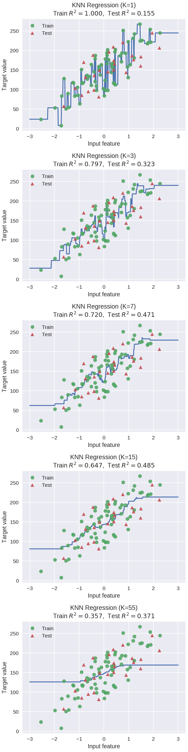
 1 # plot k-NN regression on sample dataset for different values of K
 2 fig, subaxes = plt.subplots(5, 1, figsize=(5,20))
  #生成(-3,3)区间内500个数据
 3 X_predict_input = np.linspace(-3, 3, 500).reshape(-1,1)
 4 X_train, X_test, y_train, y_test = train_test_split(X_R1, y_R1,
 5                                                    random_state = 0)
 6
 7 for thisaxis, K in zip(subaxes, [1, 3, 7, 15, 55]):
 8     knnreg = KNeighborsRegressor(n_neighbors = K).fit(X_train, y_train)
 9     y_predict_output = knnreg.predict(X_predict_input)
10     train_score = knnreg.score(X_train, y_train)
11     test_score = knnreg.score(X_test, y_test)
    #通过下面这个plot画出线条(其实是离散的点较密形成的)
12     thisaxis.plot(X_predict_input, y_predict_output)
13     thisaxis.plot(X_train, y_train, 'o', alpha=0.9, label='Train')
14     thisaxis.plot(X_test, y_test, '^', alpha=0.9, label='Test')
15     thisaxis.set_xlabel('Input feature')
16     thisaxis.set_ylabel('Target value')
17     thisaxis.set_title('KNN Regression (K={})

18 Train $R^2 = {:.3f}$,  Test $R^2 = {:.3f}$'
19                       .format(K, train_score, test_score))
20     thisaxis.legend()
21     plt.tight_layout(pad=0.4, w_pad=0.5, h_pad=1.0)
KNN参数k对回归预测的影响
线性回归预测模型
 1 from sklearn.linear_model import LinearRegression
 2
 3 X_train, X_test, y_train, y_test = train_test_split(X_R1, y_R1,
 4                                                    random_state = 0)
 5 linreg = LinearRegression().fit(X_train, y_train)
 6
 7 #coef_:偏置参数
 8 print('linear model coeff (w): {}'
 9      .format(linreg.coef_))
10 #intercept_:各个参数前面的权重
11 #(intercept_[0]*x[0]+...+intercept_[n]*x[n] = y
12 print('linear model intercept (b): {:.3f}'
13      .format(linreg.intercept_))
14 print('R-squared score (training): {:.3f}'
15      .format(linreg.score(X_train, y_train)))
16 print('R-squared score (test): {:.3f}'
17      .format(linreg.score(X_test, y_test)))
linear model coeff (w): [ 45.71]
linear model intercept (b): 148.446
R-squared score (training): 0.679
R-squared score (test): 0.492
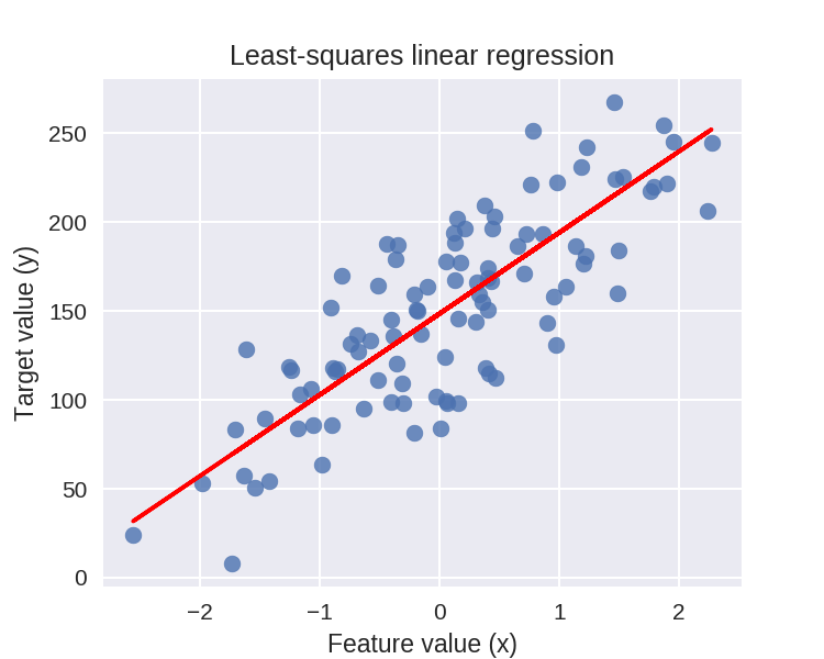
线性回归图示
1 plt.figure(figsize=(5,4))
2 plt.scatter(X_R1, y_R1, marker= 'o', s=50, alpha=0.8)
3 #画出拟合出来的直线
4 plt.plot(X_R1, linreg.coef_ * X_R1 + linreg.intercept_, 'r-')
5 plt.title('Least-squares linear regression')
6 plt.xlabel('Feature value (x)')
7 plt.ylabel('Target value (y)')
8 plt.show()
多元线性回归预测
 1 X_train, X_test, y_train, y_test = train_test_split(X_crime, y_crime,
 2                                                    random_state = 0)
 3 linreg = LinearRegression().fit(X_train, y_train)
 4
 5 print('Crime dataset')
 6 print('linear model intercept: {}'
 7      .format(linreg.intercept_))
 8 print('linear model coeff:
{}'
 9      .format(linreg.coef_))
10 print('R-squared score (training): {:.3f}'
11      .format(linreg.score(X_train, y_train)))
12 print('R-squared score (test): {:.3f}'
13      .format(linreg.score(X_test, y_test)))
linear model intercept: 3861.708902399444
linear model coeff:
[  1.62e-03  -1.03e+02   1.61e+01  -2.94e+01  -1.92e+00  -1.47e+01
  -2.41e-03   1.46e+00  -1.46e-02  -1.08e+01   4.35e+01  -6.92e+00
   4.95e+00  -4.11e+00  -3.63e+00   8.98e-03   8.33e-03   4.84e-03
  -5.25e+00  -1.59e+01   7.47e+00   2.31e+00  -2.48e-01   1.22e+01
  -2.90e+00  -1.49e+00   4.96e+00   5.21e+00   1.82e+02   1.15e+01
   1.54e+02  -3.40e+02  -1.22e+02   2.75e+00  -2.87e+01   2.39e+00
   9.44e-01   3.18e+00  -1.17e+01  -5.46e-03   4.24e+01  -1.10e-03
  -9.23e-01   5.13e+00  -4.69e+00   1.13e+00  -1.70e+01  -5.00e+01
   5.64e+01  -2.94e+01   3.42e-01  -3.10e+01   2.89e+01  -5.46e+01
   6.75e+02   8.54e+01  -3.35e+02  -3.17e+01   2.96e+01   7.07e+00
   7.46e+01   2.01e-02  -3.96e-01   3.15e+01   1.00e+01  -1.60e+00
  -5.63e-01   2.82e+00  -2.96e+01   1.08e+11  -1.01e-03  -1.08e+11
   1.08e+11  -3.13e+08  -4.95e-01   3.13e+08  -3.13e+08   1.47e+00
  -2.78e+00   1.12e+00  -3.70e+01   1.09e-01   3.07e-01   2.06e+01
   9.24e-01  -6.05e-01  -1.92e+00   5.88e-01]
R-squared score (training): 0.668
R-squared score (test): 0.520
岭回归
 1 from sklearn.linear_model import Ridge
 2 X_train, X_test, y_train, y_test = train_test_split(X_crime, y_crime,
 3                                                    random_state = 0)
 4 #alpha为岭回归的正则化系数
 5 linridge = Ridge(alpha=20.0).fit(X_train, y_train)
 6
 7 print('Crime dataset')
 8 print('ridge regression linear model intercept: {}'
 9      .format(linridge.intercept_))
10 print('ridge regression linear model coeff:
{}'
11      .format(linridge.coef_))
12 print('R-squared score (training): {:.3f}'
13      .format(linridge.score(X_train, y_train)))
14 print('R-squared score (test): {:.3f}'
15      .format(linridge.score(X_test, y_test)))
16 print('Number of non-zero features: {}'
17      .format(np.sum(linridge.coef_ != 0)))
Crime dataset
ridge regression linear model intercept: -3352.4230358464793
ridge regression linear model coeff:
[  1.95e-03   2.19e+01   9.56e+00  -3.59e+01   6.36e+00  -1.97e+01
  -2.81e-03   1.66e+00  -6.61e-03  -6.95e+00   1.72e+01  -5.63e+00
   8.84e+00   6.79e-01  -7.34e+00   6.70e-03   9.79e-04   5.01e-03
  -4.90e+00  -1.79e+01   9.18e+00  -1.24e+00   1.22e+00   1.03e+01
  -3.78e+00  -3.73e+00   4.75e+00   8.43e+00   3.09e+01   1.19e+01
  -2.05e+00  -3.82e+01   1.85e+01   1.53e+00  -2.20e+01   2.46e+00
   3.29e-01   4.02e+00  -1.13e+01  -4.70e-03   4.27e+01  -1.23e-03
   1.41e+00   9.35e-01  -3.00e+00   1.12e+00  -1.82e+01  -1.55e+01
   2.42e+01  -1.32e+01  -4.20e-01  -3.60e+01   1.30e+01  -2.81e+01
   4.39e+01   3.87e+01  -6.46e+01  -1.64e+01   2.90e+01   4.15e+00
   5.34e+01   1.99e-02  -5.47e-01   1.24e+01   1.04e+01  -1.57e+00
   3.16e+00   8.78e+00  -2.95e+01  -2.34e-04   3.14e-04  -4.13e-04
  -1.80e-04  -5.74e-01  -5.18e-01  -4.21e-01   1.53e-01   1.33e+00
   3.85e+00   3.03e+00  -3.78e+01   1.38e-01   3.08e-01   1.57e+01
   3.31e-01   3.36e+00   1.61e-01  -2.68e+00]
R-squared score (training): 0.671
R-squared score (test): 0.494
Number of non-zero features: 88


岭回归使用归一化变量
 1 from sklearn.preprocessing import MinMaxScaler
 2 scaler = MinMaxScaler()
 3
 4 from sklearn.linear_model import Ridge
 5 X_train, X_test, y_train, y_test = train_test_split(X_crime, y_crime,
 6                                                    random_state = 0)
 7
 8 #数据归一化
 9 X_train_scaled = scaler.fit_transform(X_train)
10 X_test_scaled = scaler.transform(X_test)
11
12 linridge = Ridge(alpha=20.0).fit(X_train_scaled, y_train)
13
14 print('Crime dataset')
15 print('ridge regression linear model intercept: {}'
16      .format(linridge.intercept_))
17 print('ridge regression linear model coeff:
{}'
18      .format(linridge.coef_))
19 print('R-squared score (training): {:.3f}'
20      .format(linridge.score(X_train_scaled, y_train)))
21 print('R-squared score (test): {:.3f}'
22      .format(linridge.score(X_test_scaled, y_test)))
23 print('Number of non-zero features: {}'
24      .format(np.sum(linridge.coef_ != 0)))
Crime dataset
ridge regression linear model intercept: 933.3906385044113
ridge regression linear model coeff:
[  88.69   16.49  -50.3   -82.91  -65.9    -2.28   87.74  150.95   18.88
  -31.06  -43.14 -189.44   -4.53  107.98  -76.53    2.86   34.95   90.14
   52.46  -62.11  115.02    2.67    6.94   -5.67 -101.55  -36.91   -8.71
   29.12  171.26   99.37   75.07  123.64   95.24 -330.61 -442.3  -284.5
 -258.37   17.66 -101.71  110.65  523.14   24.82    4.87  -30.47   -3.52
   50.58   10.85   18.28   44.11   58.34   67.09  -57.94  116.14   53.81
   49.02   -7.62   55.14  -52.09  123.39   77.13   45.5   184.91  -91.36
    1.08  234.09   10.39   94.72  167.92  -25.14   -1.18   14.6    36.77
   53.2   -78.86   -5.9    26.05  115.15   68.74   68.29   16.53  -97.91
  205.2    75.97   61.38  -79.83   67.27   95.67  -11.88]
R-squared score (training): 0.615
R-squared score (test): 0.599
Number of non-zero features: 88

正则化参数的岭回归的影响
 1 print('Ridge regression: effect of alpha regularization parameter
')
 2 #改变alpha(正则化参数)
 3 for this_alpha in [0, 1, 10, 20, 50, 100, 1000]:
 4     linridge = Ridge(alpha = this_alpha).fit(X_train_scaled, y_train)
 5     r2_train = linridge.score(X_train_scaled, y_train)
 6     r2_test = linridge.score(X_test_scaled, y_test)
 7     num_coeff_bigger = np.sum(abs(linridge.coef_) > 1.0)
 8     print('Alpha = {:.2f}
num abs(coeff) > 1.0: {},
 9 r-squared training: {:.2f}, r-squared test: {:.2f}
'
10          .format(this_alpha, num_coeff_bigger, r2_train, r2_test))
Ridge regression: effect of alpha regularization parameter

Alpha = 0.00
num abs(coeff) > 1.0: 87, r-squared training: 0.67, r-squared test: 0.50

Alpha = 1.00
num abs(coeff) > 1.0: 87, r-squared training: 0.66, r-squared test: 0.56

Alpha = 10.00
num abs(coeff) > 1.0: 87, r-squared training: 0.63, r-squared test: 0.59

Alpha = 20.00
num abs(coeff) > 1.0: 88, r-squared training: 0.61, r-squared test: 0.60

Alpha = 50.00
num abs(coeff) > 1.0: 86, r-squared training: 0.58, r-squared test: 0.58

Alpha = 100.00
num abs(coeff) > 1.0: 87, r-squared training: 0.55, r-squared test: 0.55

Alpha = 1000.00
num abs(coeff) > 1.0: 84, r-squared training: 0.31, r-squared test: 0.30
Lasso 回归
 1 from sklearn.linear_model import Lasso
 2 from sklearn.preprocessing import MinMaxScaler
 3 scaler = MinMaxScaler()
 4
 5 X_train, X_test, y_train, y_test = train_test_split(X_crime, y_crime,
 6                                                    random_state = 0)
 7
 8 X_train_scaled = scaler.fit_transform(X_train)
 9 X_test_scaled = scaler.transform(X_test)
10
11 linlasso = Lasso(alpha=2.0, max_iter = 10000).fit(X_train_scaled, y_train)
12
13 print('Crime dataset')
14 print('lasso regression linear model intercept: {}'
15      .format(linlasso.intercept_))
16 print('lasso regression linear model coeff:
{}'
17      .format(linlasso.coef_))
18 print('Non-zero features: {}'
19      .format(np.sum(linlasso.coef_ != 0)))
20 print('R-squared score (training): {:.3f}'
21      .format(linlasso.score(X_train_scaled, y_train)))
22 print('R-squared score (test): {:.3f}
'
23      .format(linlasso.score(X_test_scaled, y_test)))
24 print('Features with non-zero weight (sorted by absolute magnitude):')
25
26 for e in sorted (list(zip(list(X_crime), linlasso.coef_)),
27                 key = lambda e: -abs(e[1])):
28     if e[1] != 0:
29         print('	{}, {:.3f}'.format(e[0], e[1]))
Crime dataset
lasso regression linear model intercept: 1186.6120619985809
lasso regression linear model coeff:
[    0.       0.      -0.    -168.18    -0.      -0.       0.     119.69
     0.      -0.       0.    -169.68    -0.       0.      -0.       0.
     0.       0.      -0.      -0.       0.      -0.       0.       0.
   -57.53    -0.      -0.       0.     259.33    -0.       0.       0.
     0.      -0.   -1188.74    -0.      -0.      -0.    -231.42     0.
  1488.37     0.      -0.      -0.      -0.       0.       0.       0.
     0.       0.      -0.       0.      20.14     0.       0.       0.
     0.       0.     339.04     0.       0.     459.54    -0.       0.
   122.69    -0.      91.41     0.      -0.       0.       0.      73.14
     0.      -0.       0.       0.      86.36     0.       0.       0.
  -104.57   264.93     0.      23.45   -49.39     0.       5.2      0.  ]
Non-zero features: 20
R-squared score (training): 0.631
R-squared score (test): 0.624

Features with non-zero weight (sorted by absolute magnitude):
	PctKidsBornNeverMar, 1488.365
	PctKids2Par, -1188.740
	HousVacant, 459.538
	PctPersDenseHous, 339.045
	NumInShelters, 264.932
	MalePctDivorce, 259.329
	PctWorkMom, -231.423
	pctWInvInc, -169.676
	agePct12t29, -168.183
	PctVacantBoarded, 122.692
	pctUrban, 119.694
	MedOwnCostPctIncNoMtg, -104.571
	MedYrHousBuilt, 91.412
	RentQrange, 86.356
	OwnOccHiQuart, 73.144
	PctEmplManu, -57.530
	PctBornSameState, -49.394
	PctForeignBorn, 23.449
	PctLargHouseFam, 20.144
	PctSameCity85, 5.198

k(正则化系数)对Lasso回归的影响
 1 print('Lasso regression: effect of alpha regularization

 2 parameter on number of features kept in final model
')
 3
 4 for alpha in [0.5, 1, 2, 3, 5, 10, 20, 50]:
 5     linlasso = Lasso(alpha, max_iter = 10000).fit(X_train_scaled, y_train)
 6     r2_train = linlasso.score(X_train_scaled, y_train)
 7     r2_test = linlasso.score(X_test_scaled, y_test)
 8
 9     print('Alpha = {:.2f}
Features kept: {}, r-squared training: {:.2f},
10 r-squared test: {:.2f}
'
11          .format(alpha, np.sum(linlasso.coef_ != 0), r2_train, r2_test))
Lasso regression: effect of alpha regularization
parameter on number of features kept in final model

Alpha = 0.50
Features kept: 35, r-squared training: 0.65, r-squared test: 0.58

Alpha = 1.00
Features kept: 25, r-squared training: 0.64, r-squared test: 0.60

Alpha = 2.00
Features kept: 20, r-squared training: 0.63, r-squared test: 0.62

Alpha = 3.00
Features kept: 17, r-squared training: 0.62, r-squared test: 0.63

Alpha = 5.00
Features kept: 12, r-squared training: 0.60, r-squared test: 0.61

Alpha = 10.00
Features kept: 6, r-squared training: 0.57, r-squared test: 0.58

Alpha = 20.00
Features kept: 2, r-squared training: 0.51, r-squared test: 0.50

Alpha = 50.00
Features kept: 1, r-squared training: 0.31, r-squared test: 0.30

多元回归
 1 from sklearn.linear_model import LinearRegression
 2 from sklearn.linear_model import Ridge
 3 from sklearn.preprocessing import PolynomialFeatures
 4
 5
 6 X_train, X_test, y_train, y_test = train_test_split(X_F1, y_F1,
 7                                                    random_state = 0)
 8 linreg = LinearRegression().fit(X_train, y_train)
 9
10 print('linear model coeff (w): {}'
11      .format(linreg.coef_))
12 print('linear model intercept (b): {:.3f}'
13      .format(linreg.intercept_))
14 print('R-squared score (training): {:.3f}'
15      .format(linreg.score(X_train, y_train)))
16 print('R-squared score (test): {:.3f}'
17      .format(linreg.score(X_test, y_test)))
18
19 print('对参数开方,使参数变成平方的表示形式')
20 poly = PolynomialFeatures(degree=2)
21 X_F1_poly = poly.fit_transform(X_F1)
22
23 X_train, X_test, y_train, y_test = train_test_split(X_F1_poly, y_F1,
24                                                    random_state = 0)
25 linreg = LinearRegression().fit(X_train, y_train)
26
27 print('(poly deg 2) linear model coeff (w):
{}'
28      .format(linreg.coef_))
29 print('(poly deg 2) linear model intercept (b): {:.3f}'
30      .format(linreg.intercept_))
31 print('(poly deg 2) R-squared score (training): {:.3f}'
32      .format(linreg.score(X_train, y_train)))
33 print('(poly deg 2) R-squared score (test): {:.3f}
'
34      .format(linreg.score(X_test, y_test)))
35
36 print('使用平方的参数,会很容易导致过拟合,通过对平方参数加上

37 正则化,减少过拟合情况,类似岭回归')
38
39 X_train, X_test, y_train, y_test = train_test_split(X_F1_poly, y_F1,
40                                                    random_state = 0)
41 linreg = Ridge().fit(X_train, y_train)
42
43 print('(poly deg 2 + ridge) linear model coeff (w):
{}'
44      .format(linreg.coef_))
45 print('(poly deg 2 + ridge) linear model intercept (b): {:.3f}'
46      .format(linreg.intercept_))
47 print('(poly deg 2 + ridge) R-squared score (training): {:.3f}'
48      .format(linreg.score(X_train, y_train)))
49 print('(poly deg 2 + ridge) R-squared score (test): {:.3f}'
50      .format(linreg.score(X_test, y_test)))
linear model coeff (w): [ 4.42 6. 0.53 10.24 6.55 -2.02 -0.32] linear model intercept (b): 1.543 R-squared score (training): 0.722 R-squared score (test): 0.722 对参数开方,使参数变成平方的表示形式 (poly deg 2) linear model coeff (w): [ 3.41e-12 1.66e+01 2.67e+01 -2.21e+01 1.24e+01 6.93e+00 1.05e+00 3.71e+00 -1.34e+01 -5.73e+00 1.62e+00 3.66e+00 5.05e+00 -1.46e+00 1.95e+00 -1.51e+01 4.87e+00 -2.97e+00 -7.78e+00 5.15e+00 -4.65e+00 1.84e+01 -2.22e+00 2.17e+00 -1.28e+00 1.88e+00 1.53e-01 5.62e-01 -8.92e-01 -2.18e+00 1.38e+00 -4.90e+00 -2.24e+00 1.38e+00 -5.52e-01 -1.09e+00] (poly deg 2) linear model intercept (b): -3.206 (poly deg 2) R-squared score (training): 0.969 (poly deg 2) R-squared score (test): 0.805 使用平方的参数,会很容易导致过拟合,通过对平方参数加上 正则化,减少过拟合情况,类似岭回归 (poly deg 2 + ridge) linear model coeff (w): [ 0. 2.23 4.73 -3.15 3.86 1.61 -0.77 -0.15 -1.75 1.6 1.37 2.52 2.72 0.49 -1.94 -1.63 1.51 0.89 0.26 2.05 -1.93 3.62 -0.72 0.63 -3.16 1.29 3.55 1.73 0.94 -0.51 1.7 -1.98 1.81 -0.22 2.88 -0.89] (poly deg 2 + ridge) linear model intercept (b): 5.418 (poly deg 2 + ridge) R-squared score (training): 0.826 (poly deg 2 + ridge) R-squared score (test): 0.825
线性模型用于分类
逻辑回归
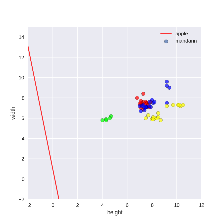
使用高度,跨度作为参数进行水果类型分类
 1 from sklearn.linear_model import LogisticRegression
 2 from adspy_shared_utilities import (
 3 plot_class_regions_for_classifier_subplot)
 4
 5 fig, subaxes = plt.subplots(1, 1, figsize=(7, 5))
 6 y_fruits_apple = y_fruits_2d == 1   # make into a binary problem: apples vs everything else
  #as_matrix()把表格转化成矩阵,方便计算
 7 X_train, X_test, y_train, y_test = (
 8 train_test_split(X_fruits_2d.as_matrix(),
 9                 y_fruits_apple.as_matrix(),
10                 random_state = 0))
11
12 clf = LogisticRegression(C=100).fit(X_train, y_train)
13 plot_class_regions_for_classifier_subplot(clf, X_train, y_train, None,
14                                          None, 'Logistic regression
15 for binary classification
Fruit dataset: Apple vs others',
16                                          subaxes)
17
18 h = 6
19 w = 8
20 print('A fruit with height {} and width {} is predicted to be: {}'
21      .format(h,w, ['not an apple', 'an apple'][clf.predict([[h,w]])[0]]))
22
23 h = 10
24 w = 7
25 print('A fruit with height {} and width {} is predicted to be: {}'
26      .format(h,w, ['not an apple', 'an apple'][clf.predict([[h,w]])[0]]))
27 subaxes.set_xlabel('height')
28 subaxes.set_ylabel('width')
29
30 print('Accuracy of Logistic regression classifier on training set: {:.2f}'
31      .format(clf.score(X_train, y_train)))
32 print('Accuracy of Logistic regression classifier on test set: {:.2f}'
33      .format(clf.score(X_test, y_test)))

A fruit with height 6 and width 8 is predicted to be: an apple
A fruit with height 10 and width 7 is predicted to be: not an apple
Accuracy of Logistic regression classifier on training set: 0.77
Accuracy of Logistic regression classifier on test set: 0.73
 1 from sklearn.linear_model import LogisticRegression
 2 from adspy_shared_utilities import (
 3 plot_class_regions_for_classifier_subplot)
 4
 5
 6 X_train, X_test, y_train, y_test = train_test_split(X_C2, y_C2,
 7                                                    random_state = 0)
 8
 9 fig, subaxes = plt.subplots(1, 1, figsize=(7, 5))
10 clf = LogisticRegression().fit(X_train, y_train)
11 title = 'Logistic regression, simple synthetic dataset C = {:.3f}'.format(1.0)
12 plot_class_regions_for_classifier_subplot(clf, X_train, y_train,
13                                          None, None, title, subaxes)
14
15 print('Accuracy of Logistic regression classifier on training set: {:.2f}'
16      .format(clf.score(X_train, y_train)))
17 print('Accuracy of Logistic regression classifier on test set: {:.2f}'
18      .format(clf.score(X_test, y_test)))
19
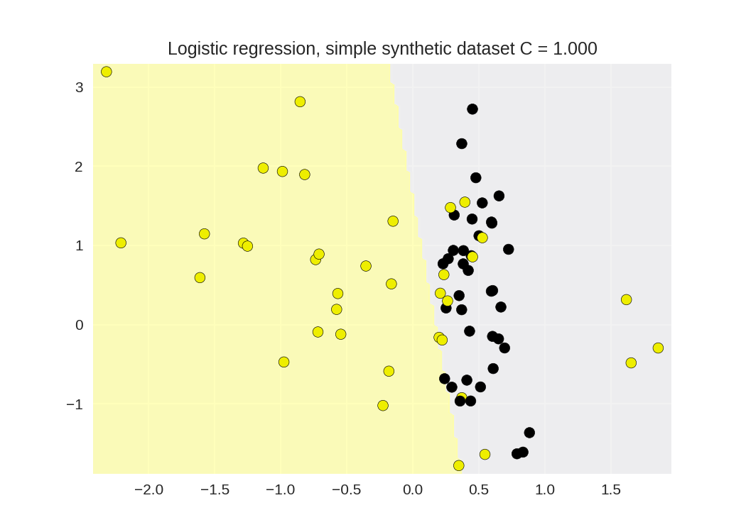
Accuracy of Logistic regression classifier on training set: 0.80
Accuracy of Logistic regression classifier on test set: 0.80
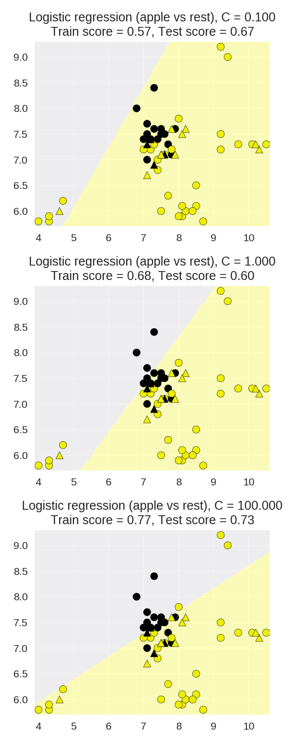
逻辑回归正则化参数的影响
 1 X_train, X_test, y_train, y_test = (
 2 train_test_split(X_fruits_2d.as_matrix(),
 3                 y_fruits_apple.as_matrix(),
 4                 random_state=0))
 5
 6 fig, subaxes = plt.subplots(3, 1, figsize=(4, 10))
 7
 8 for this_C, subplot in zip([0.1, 1, 100], subaxes):
 9     clf = LogisticRegression(C=this_C).fit(X_train, y_train)
10     title ='Logistic regression (apple vs rest), C = {:.3f}'.format(this_C)
11
12     plot_class_regions_for_classifier_subplot(clf, X_train, y_train,
13                                              X_test, y_test, title,
14                                              subplot)
15 plt.tight_layout()
应用于真实数据
 1 from sklearn.linear_model import LogisticRegression
 2
 3 X_train, X_test, y_train, y_test = train_test_split(X_cancer, y_cancer, random_state = 0)
 4
 5 clf = LogisticRegression().fit(X_train, y_train)
 6 print('Breast cancer dataset')
 7 print('Accuracy of Logistic regression classifier on training set: {:.2f}'
 8      .format(clf.score(X_train, y_train)))
 9 print('Accuracy of Logistic regression classifier on test set: {:.2f}'
10      .format(clf.score(X_test, y_test)))
Breast cancer dataset
Accuracy of Logistic regression classifier on training set: 0.96
Accuracy of Logistic regression classifier on test set: 0.96
SVM
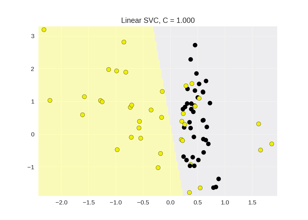
线性SVM
 1 from sklearn.svm import SVC
 2 from adspy_shared_utilities import plot_class_regions_for_classifier_subplot
 3
 4
 5 X_train, X_test, y_train, y_test = train_test_split(X_C2, y_C2, random_state = 0)
 6
 7 fig, subaxes = plt.subplots(1, 1, figsize=(7, 5))
 8 this_C = 1.0
 9 #线性核函数
10 clf = SVC(kernel = 'linear', C=this_C).fit(X_train, y_train)
11 title = 'Linear SVC, C = {:.3f}'.format(this_C)
12 plot_class_regions_for_classifier_subplot(clf, X_train, y_train, None, None, title, subaxes)
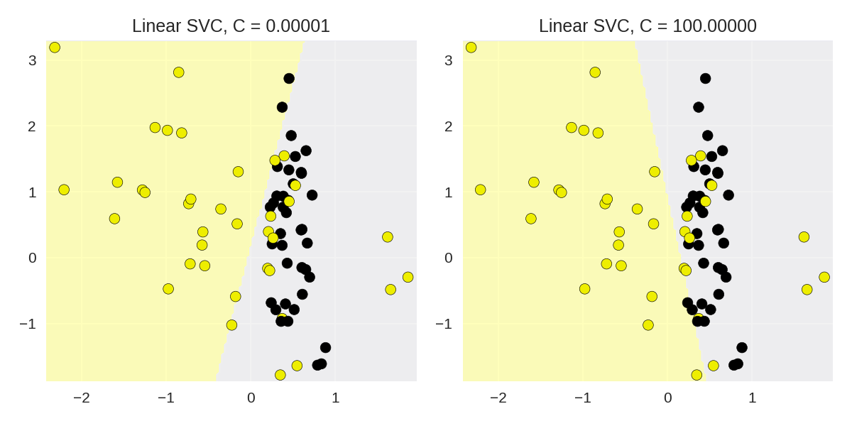
Linear Support Vector Machine: C parameter
 1 from sklearn.svm import LinearSVC
 2 from adspy_shared_utilities import plot_class_regions_for_classifier
 3
 4 X_train, X_test, y_train, y_test = train_test_split(X_C2, y_C2, random_state = 0)
 5 fig, subaxes = plt.subplots(1, 2, figsize=(8, 4))
 6
 7 for this_C, subplot in zip([0.00001, 100], subaxes):
 8     clf = LinearSVC(C=this_C).fit(X_train, y_train)
 9     title = 'Linear SVC, C = {:.5f}'.format(this_C)
10     plot_class_regions_for_classifier_subplot(clf, X_train, y_train,
11                                              None, None, title, subplot)
12 plt.tight_layout()
线性SVM使用于真实数据
1 from sklearn.svm import LinearSVC
2 X_train, X_test, y_train, y_test = train_test_split(X_cancer, y_cancer, random_state = 0)
3
4 clf = LinearSVC().fit(X_train, y_train)
5 print('Breast cancer dataset')
6 print('Accuracy of Linear SVC classifier on training set: {:.2f}'
7      .format(clf.score(X_train, y_train)))
8 print('Accuracy of Linear SVC classifier on test set: {:.2f}'
9      .format(clf.score(X_test, y_test)))
Breast cancer dataset
Accuracy of Linear SVC classifier on training set: 0.74
Accuracy of Linear SVC classifier on test set: 0.74
使用线性模型进行多分类任务
1 from sklearn.svm import LinearSVC
2
3 X_train, X_test, y_train, y_test = train_test_split(X_fruits_2d, y_fruits_2d, random_state = 0)
4
5 clf = LinearSVC(C=5, random_state = 67).fit(X_train, y_train)
6 print('Coefficients:
', clf.coef_)
7 print('Intercepts:
', clf.intercept_)
Coefficients:
 [[-0.26  0.71]
 [-1.63  1.16]
 [ 0.03  0.29]
 [ 1.24 -1.64]]
Intercepts:
 [-3.29  1.2  -2.72  1.16]
在水果数据集上使用多分类
 1 plt.figure(figsize=(6,6))
 2 colors = ['r', 'g', 'b', 'y']
 3 cmap_fruits = ListedColormap(['#FF0000', '#00FF00', '#0000FF','#FFFF00'])
 4
 5 plt.scatter(X_fruits_2d[['height']], X_fruits_2d[['width']],
 6            c=y_fruits_2d, cmap=cmap_fruits, edgecolor = 'black', alpha=.7)
 7
 8 x_0_range = np.linspace(-10, 15)
 9
10 for w, b, color in zip(clf.coef_, clf.intercept_, ['r', 'g', 'b', 'y']):
11     # Since class prediction with a linear model uses the formula y = w_0 x_0 + w_1 x_1 + b,
12     # and the decision boundary is defined as being all points with y = 0, to plot x_1 as a
13     # function of x_0 we just solve w_0 x_0 + w_1 x_1 + b = 0 for x_1:
14     plt.plot(x_0_range, -(x_0_range * w[0] + b) / w[1], c=color, alpha=.8)
15
16 plt.legend(target_names_fruits)
17 plt.xlabel('height')
18 plt.ylabel('width')
19 plt.xlim(-2, 12)
20 plt.ylim(-2, 15)
21 plt.show()
核化SVM
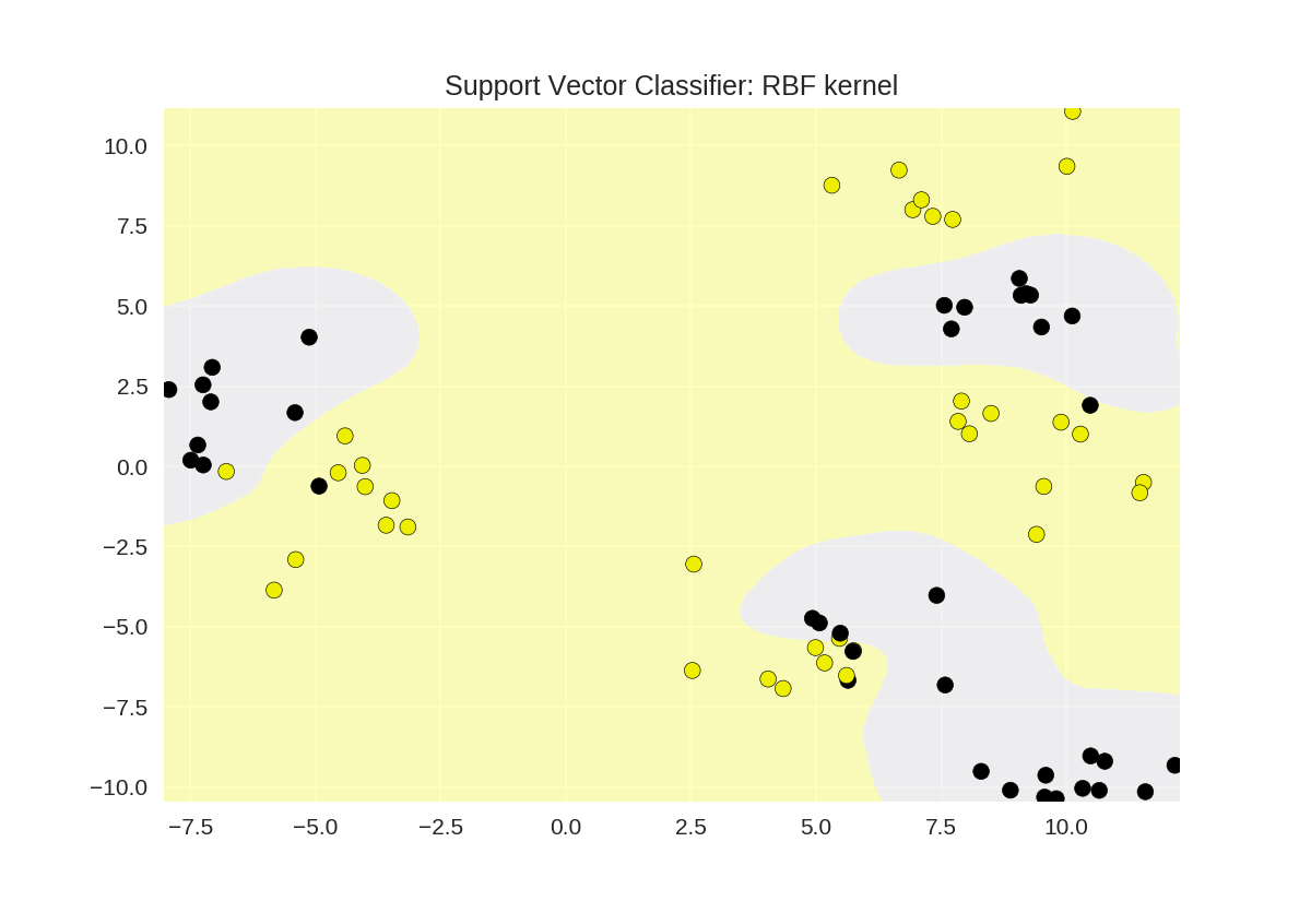
分类模型
 1 from sklearn.svm import SVC
 2 from adspy_shared_utilities import plot_class_regions_for_classifier
 3
 4 X_train, X_test, y_train, y_test = train_test_split(X_D2, y_D2, random_state = 0)
 5
 6 # RBF核函数
 7 plot_class_regions_for_classifier(SVC().fit(X_train, y_train),
 8                                  X_train, y_train, None, None,
 9                                  'Support Vector Classifier: RBF kernel')
10
11 # 多项式核函数polynomial kernel, degree = 3
12 plot_class_regions_for_classifier(SVC(kernel = 'poly', degree = 3)
13                                  .fit(X_train, y_train), X_train,
14                                  y_train, None, None,
15                                  'Support Vector Classifier: Polynomial kernel, degree = 3')

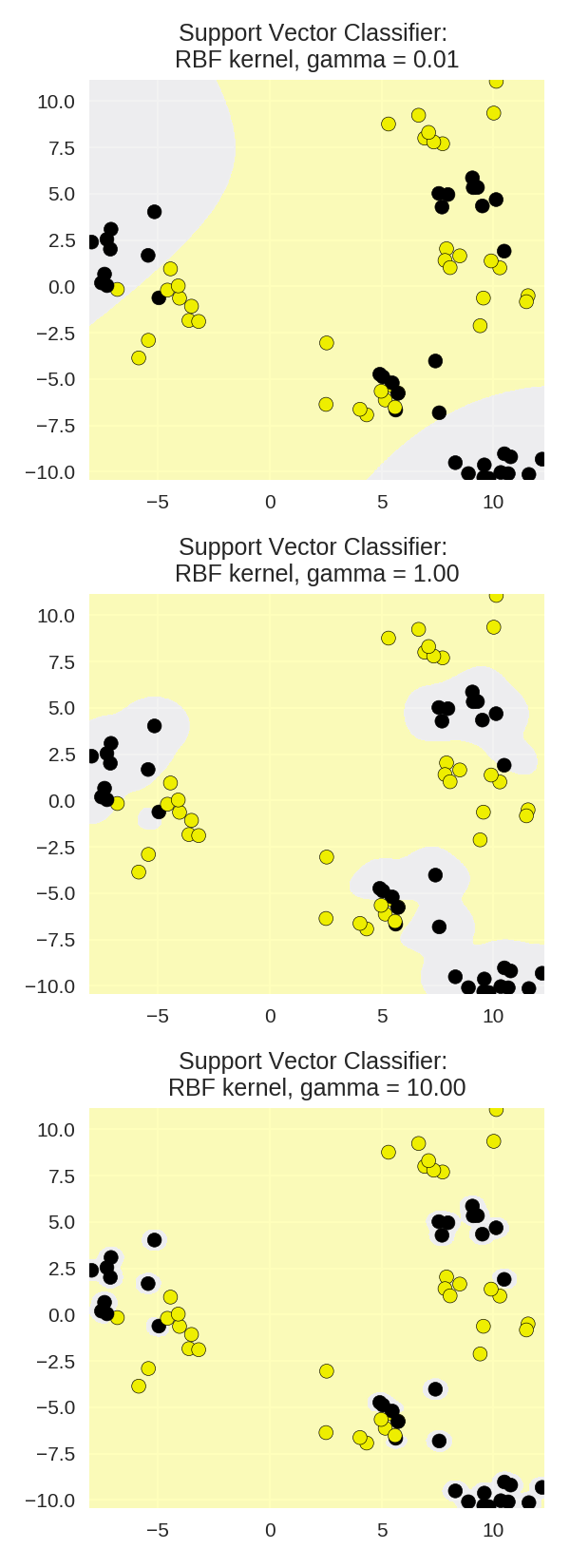
γ参数对RBF核函数SVM的影响
 1 from adspy_shared_utilities import plot_class_regions_for_classifier
 2
 3 X_train, X_test, y_train, y_test = train_test_split(X_D2, y_D2, random_state = 0)
 4 fig, subaxes = plt.subplots(3, 1, figsize=(4, 11))
 5
 6 for this_gamma, subplot in zip([0.01, 1.0, 10.0], subaxes):
 7     clf = SVC(kernel = 'rbf', gamma=this_gamma).fit(X_train, y_train)
 8     title = 'Support Vector Classifier:
RBF kernel, gamma = {:.2f}'.format(this_gamma)
 9     plot_class_regions_for_classifier_subplot(clf, X_train, y_train,
10                                              None, None, title, subplot)
11     plt.tight_layout()
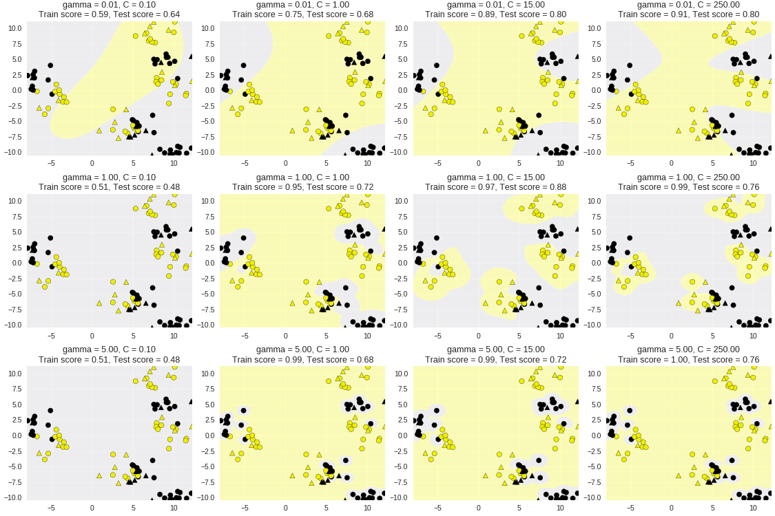
γ和C对RBP核函数SVM的影响
 1 from sklearn.svm import SVC
 2 from adspy_shared_utilities import plot_class_regions_for_classifier_subplot
 3
 4 from sklearn.model_selection import train_test_split
 5
 6
 7 X_train, X_test, y_train, y_test = train_test_split(X_D2, y_D2, random_state = 0)
 8 fig, subaxes = plt.subplots(3, 4, figsize=(15, 10), dpi=50)
 9
10 for this_gamma, this_axis in zip([0.01, 1, 5], subaxes):
11
12     for this_C, subplot in zip([0.1, 1, 15, 250], this_axis):
13         title = 'gamma = {:.2f}, C = {:.2f}'.format(this_gamma, this_C)
14         clf = SVC(kernel = 'rbf', gamma = this_gamma,
15                  C = this_C).fit(X_train, y_train)
16         plot_class_regions_for_classifier_subplot(clf, X_train, y_train,
17                                                  X_test, y_test, title,
18                                                  subplot)
19         plt.tight_layout(pad=0.4, w_pad=0.5, h_pad=1.0)
非标准化数据应用于SVM
 1 from sklearn.svm import SVC
 2 X_train, X_test, y_train, y_test = train_test_split(X_cancer, y_cancer,
 3                                                    random_state = 0)
 4
 5 clf = SVC(C=10).fit(X_train, y_train)
 6 print('Breast cancer dataset (unnormalized features)')
 7 print('Accuracy of RBF-kernel SVC on training set: {:.2f}'
 8      .format(clf.score(X_train, y_train)))
 9 print('Accuracy of RBF-kernel SVC on test set: {:.2f}'
10      .format(clf.score(X_test, y_test)))
Breast cancer dataset (unnormalized features)
Accuracy of RBF-kernel SVC on training set: 1.00
Accuracy of RBF-kernel SVC on test set: 0.63
SVM应用于标准化数据
 1 from sklearn.preprocessing import MinMaxScaler
 2 scaler = MinMaxScaler()
 3 X_train_scaled = scaler.fit_transform(X_train)
 4 X_test_scaled = scaler.transform(X_test)
 5
 6 clf = SVC(C=10).fit(X_train_scaled, y_train)
 7 print('Breast cancer dataset (normalized with MinMax scaling)')
 8 print('RBF-kernel SVC (with MinMax scaling) training set accuracy: {:.2f}'
 9      .format(clf.score(X_train_scaled, y_train)))
10 print('RBF-kernel SVC (with MinMax scaling) test set accuracy: {:.2f}'
11      .format(clf.score(X_test_scaled, y_test)))
Breast cancer dataset (normalized with MinMax scaling)
RBF-kernel SVC (with MinMax scaling) training set accuracy: 0.98
RBF-kernel SVC (with MinMax scaling) test set accuracy: 0.96
交叉验证
 1 from sklearn.model_selection import cross_val_score
 2
 3 clf = KNeighborsClassifier(n_neighbors = 5)
 4 X = X_fruits_2d.as_matrix()
 5 y = y_fruits_2d.as_matrix()
 6 #进行交叉验证
 7 cv_scores = cross_val_score(clf, X, y)
 8
 9 print('Cross-validation scores (3-fold):', cv_scores)
10 print('Mean cross-validation score (3-fold): {:.3f}'
11      .format(np.mean(cv_scores)))
Cross-validation scores (3-fold): [ 0.77  0.74  0.83]
Mean cross-validation score (3-fold): 0.781
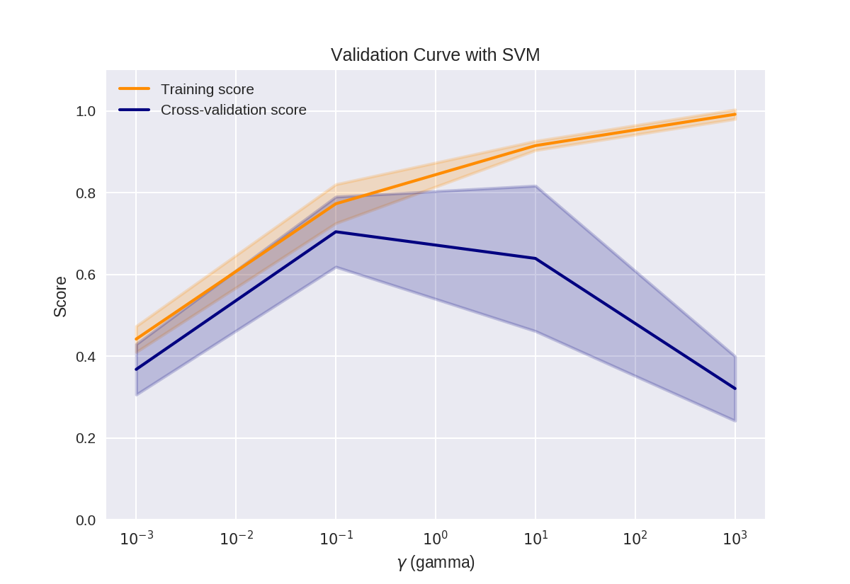
验证曲线
1 from sklearn.svm import SVC
2 from sklearn.model_selection import validation_curve
3
4 param_range = np.logspace(-3, 3, 4)
5 train_scores, test_scores = validation_curve(SVC(), X, y,
6                                             param_name='gamma',
7                                             param_range=param_range, cv=3)
1 print(train_scores)
[[ 0.49  0.42  0.41]
 [ 0.84  0.72  0.76]
 [ 0.92  0.9   0.93]
 [ 1.    1.    0.98]]
1 print(test_scores)
[[ 0.45  0.32  0.33]
 [ 0.82  0.68  0.61]
 [ 0.41  0.84  0.67]
 [ 0.36  0.21  0.39]]
 1 # This code based on scikit-learn validation_plot example
 2 #  See:  http://scikit-learn.org/stable/auto_examples/model_selection/plot_validation_curve.html
 3 plt.figure()
 4
 5 train_scores_mean = np.mean(train_scores, axis=1)
 6 train_scores_std = np.std(train_scores, axis=1)
 7 test_scores_mean = np.mean(test_scores, axis=1)
 8 test_scores_std = np.std(test_scores, axis=1)
 9
10 plt.title('Validation Curve with SVM')
11 plt.xlabel('$gamma$ (gamma)')
12 plt.ylabel('Score')
13 plt.ylim(0.0, 1.1)
14 lw = 2
15
16 plt.semilogx(param_range, train_scores_mean, label='Training score',
17             color='darkorange', lw=lw)
18
19 plt.fill_between(param_range, train_scores_mean - train_scores_std,
20                 train_scores_mean + train_scores_std, alpha=0.2,
21                 color='darkorange', lw=lw)
22
23 plt.semilogx(param_range, test_scores_mean, label='Cross-validation score',
24             color='navy', lw=lw)
25
26 plt.fill_between(param_range, test_scores_mean - test_scores_std,
27                 test_scores_mean + test_scores_std, alpha=0.2,
28                 color='navy', lw=lw)
29
30 plt.legend(loc='best')
31 plt.show()
决策树
 1 from sklearn.datasets import load_iris
 2 from sklearn.tree import DecisionTreeClassifier
 3 from adspy_shared_utilities import plot_decision_tree
 4 from sklearn.model_selection import train_test_split
 5
 6
 7 iris = load_iris()
 8
 9 X_train, X_test, y_train, y_test = train_test_split(iris.data, iris.target, random_state = 3)
10 clf = DecisionTreeClassifier().fit(X_train, y_train)
11
12 print('Accuracy of Decision Tree classifier on training set: {:.2f}'
13      .format(clf.score(X_train, y_train)))
14 print('Accuracy of Decision Tree classifier on test set: {:.2f}'
15      .format(clf.score(X_test, y_test)))
设置树的深度避免过拟合
#max_depth设置决策树的最大深度
1 clf2 = DecisionTreeClassifier(max_depth = 3).fit(X_train, y_train)
2
3 print('Accuracy of Decision Tree classifier on training set: {:.2f}'
4      .format(clf2.score(X_train, y_train)))
5 print('Accuracy of Decision Tree classifier on test set: {:.2f}'
6      .format(clf2.score(X_test, y_test)))
Accuracy of Decision Tree classifier on training set: 0.98
Accuracy of Decision Tree classifier on test set: 0.97
可视化决策树
1 plot_decision_tree(clf, iris.feature_names, iris.target_names)
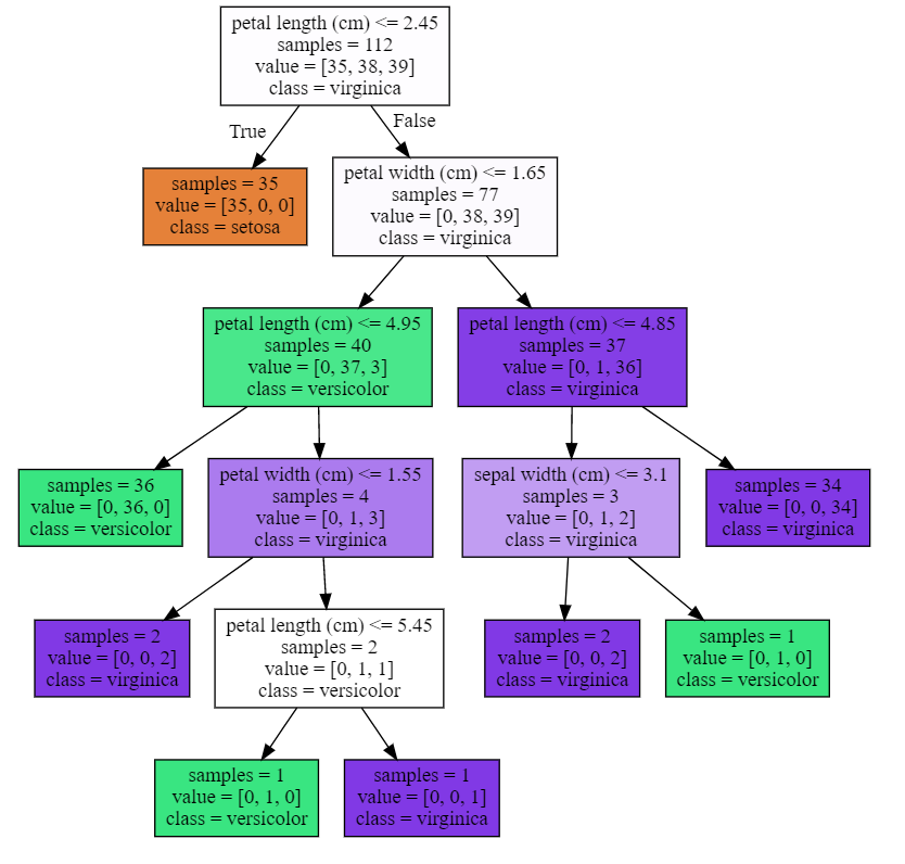
1 #决策树的最大深度为3
2 plot_decision_tree(clf2, iris.feature_names, iris.target_names)

变量的重要性
1 from adspy_shared_utilities import plot_feature_importances
2
3 plt.figure(figsize=(10,4), dpi=80)
4 plot_feature_importances(clf, iris.feature_names)
5 plt.show()
6
7 print('Feature importances: {}'.format(clf.feature_importances_))
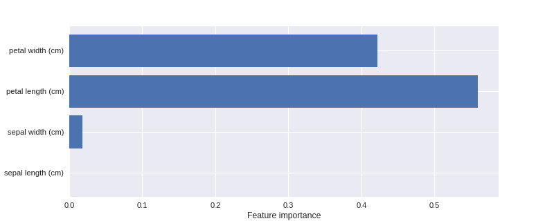
Feature importances: [ 0. 0.02 0.56 0.42]
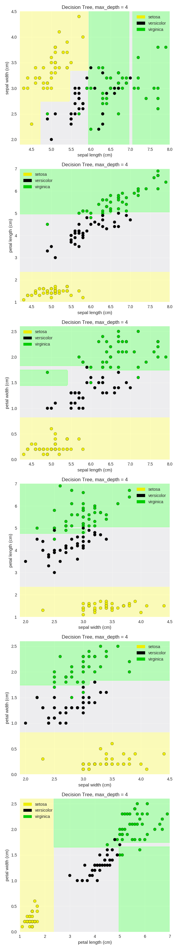
 1 from sklearn.tree import DecisionTreeClassifier
 2 from adspy_shared_utilities import plot_class_regions_for_classifier_subplot
 3
 4 X_train, X_test, y_train, y_test = train_test_split(iris.data, iris.target, random_state = 0)
 5 fig, subaxes = plt.subplots(6, 1, figsize=(6, 32))
 6
 7 pair_list = [[0,1], [0,2], [0,3], [1,2], [1,3], [2,3]]
 8 tree_max_depth = 4
 9
10 for pair, axis in zip(pair_list, subaxes):
11     X = X_train[:, pair]
12     y = y_train
13
14     clf = DecisionTreeClassifier(max_depth=tree_max_depth).fit(X, y)
15     title = 'Decision Tree, max_depth = {:d}'.format(tree_max_depth)
16     plot_class_regions_for_classifier_subplot(clf, X, y, None,
17                                              None, title, axis,
18                                              iris.target_names)
19
20     axis.set_xlabel(iris.feature_names[pair[0]])
21     axis.set_ylabel(iris.feature_names[pair[1]])
22
23 plt.tight_layout()
24 plt.show()
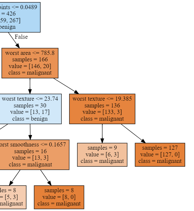
决策树应用于真实数据
 1 from sklearn.tree import DecisionTreeClassifier
 2 from adspy_shared_utilities import plot_decision_tree
 3 from adspy_shared_utilities import plot_feature_importances
 4
 5 X_train, X_test, y_train, y_test = train_test_split(X_cancer, y_cancer, random_state = 0)
 6
 7 clf = DecisionTreeClassifier(max_depth = 4, min_samples_leaf = 8,
 8                             random_state = 0).fit(X_train, y_train)
 9
10 plot_decision_tree(clf, cancer.feature_names, cancer.target_names)

 1 print('Breast cancer dataset: decision tree')
 2 print('Accuracy of DT classifier on training set: {:.2f}'
 3      .format(clf.score(X_train, y_train)))
 4 print('Accuracy of DT classifier on test set: {:.2f}'
 5      .format(clf.score(X_test, y_test)))
 6
 7 plt.figure(figsize=(10,6),dpi=80)
 8 plot_feature_importances(clf, cancer.feature_names)
 9 plt.tight_layout()
10
11 plt.show()
Breast cancer dataset: decision tree
Accuracy of DT classifier on training set: 0.96
Accuracy of DT classifier on test set: 0.94
