第十三节，使用带有全局平均池化层的CNN对CIFAR10数据集分类

这里使用的数据集仍然是CIFAR-10，由于之前写过一篇使用AlexNet对CIFAR数据集进行分类的文章，已经详细介绍了这个数据集，当时我们是直接把这些图片的数据文件下载下来，然后使用pickle进行反序列化获取数据的，具体内容可以参考这里：第十六节，卷积神经网络之AlexNet网络实现(六)

与MNIST类似，TensorFlow中也有一个下载和导入CIFAR数据集的代码文件，不同的是，自从TensorFlow1.0之后，将里面的Models模块分离了出来，分离和导入CIFAR数据集的代码在models中，所以要先去TensorFlow的GitHub网站将其下载下来。点击下载地址开始下载。

一 描述

在该例子中，使用了全局平均池化层来代替传统的全连接层，使用了3个卷积层的同卷积网络，滤波器为5x5，每个卷积层后面跟有一个步长2x2的池化层，滤波器大小为2x2,最后一个池化层为全局平均池化层，输出后为batch_sizex1x1x10，我们对其进行形状变换为batch_sizex10，得到10个特征，再对这10个特征进行softmax计算，其结果代表最终分类。

• 输入图片大小为24x24x3
• 经过5x5的同卷积操作(步长为1)，输出64个通道，得到24x24x64的输出
• 经过f=2,s=2的池化层，得到大小为12x12x24的输出
• 经过5x5的同卷积操作(步长为1)，输出64个通道，得到12x12x64的输出
• 经过f=2,s=2的池化层，得到大小为6x6x64的输出
• 经过5x5的同卷积操作(步长为1)，输出10个通道，得到6x6x10的输出
• 经过一个全局平均池化层f=6,s=6，得到1x1x10的输出
• 展开成1x10的形状，经过softmax函数计算，进行分类

二 导入数据集

'''
一 引入数据集
'''
batch_size = 128
learning_rate = 1e-4
training_step = 15000
display_step = 200
#数据集目录
data_dir = './cifar10_data/cifar-10-batches-bin'
print('begin')
#获取训练集数据
images_train,labels_train = cifar10_input.inputs(eval_data=False,data_dir = data_dir,batch_size=batch_size)
print('begin data')

注意这里调用了cifar10_input.inputs()函数，这个函数是专门获取数据的函数，返回数据集合对应的标签，但是这个函数会将图片裁切好，由原来的32x32x3变成24x24x3，该函数默认使用测试数据集，如果使用训练数据集，可以将第一个参数传入eval_data=False。另外再将batch_size和dir传入，就可以得到dir下面的batch_size个数据了。我们可以查看一下这个函数的实现：

def inputs(eval_data, data_dir, batch_size):
  """Construct input for CIFAR evaluation using the Reader ops.

  Args:
    eval_data: bool, indicating if one should use the train or eval data set.
    data_dir: Path to the CIFAR-10 data directory.
    batch_size: Number of images per batch.

  Returns:
    images: Images. 4D tensor of [batch_size, IMAGE_SIZE, IMAGE_SIZE, 3] size.
    labels: Labels. 1D tensor of [batch_size] size.
  """
  if not eval_data:
    filenames = [os.path.join(data_dir, 'data_batch_%d.bin' % i)
                 for i in xrange(1, 6)]
    num_examples_per_epoch = NUM_EXAMPLES_PER_EPOCH_FOR_TRAIN
  else:
    filenames = [os.path.join(data_dir, 'test_batch.bin')]
    num_examples_per_epoch = NUM_EXAMPLES_PER_EPOCH_FOR_EVAL

  for f in filenames:
    if not tf.gfile.Exists(f):
      raise ValueError('Failed to find file: ' + f)

  with tf.name_scope('input'):
    # Create a queue that produces the filenames to read.
    filename_queue = tf.train.string_input_producer(filenames)

    # Read examples from files in the filename queue.
    read_input = read_cifar10(filename_queue)
    reshaped_image = tf.cast(read_input.uint8image, tf.float32)

    height = IMAGE_SIZE
    width = IMAGE_SIZE

    # Image processing for evaluation.
    # Crop the central [height, width] of the image.
    resized_image = tf.image.resize_image_with_crop_or_pad(reshaped_image,
                                                           height, width)

    # Subtract off the mean and divide by the variance of the pixels.
    float_image = tf.image.per_image_standardization(resized_image)

    # Set the shapes of tensors.
    float_image.set_shape([height, width, 3])
    read_input.label.set_shape([1])

    # Ensure that the random shuffling has good mixing properties.
    min_fraction_of_examples_in_queue = 0.4
    min_queue_examples = int(num_examples_per_epoch *
                             min_fraction_of_examples_in_queue)

  # Generate a batch of images and labels by building up a queue of examples.
  return _generate_image_and_label_batch(float_image, read_input.label,
                                         min_queue_examples, batch_size,
                                         shuffle=False)

 这个函数主要包含以下几步：

• 读取测试集文件名或者训练集文件名，并创建文件名队列。
• 使用文件读取器读取一张图像的数据和标签，并返回一个存放这些张量数据的类对象。
• 对图像进行裁切处理。
• 归一化输入。
• 读取batch_size个图像和标签。(返回的是一个张量，必须要在会话中执行才能得到数据)

三 定义网络结构

'''
二 定义网络结构
'''
def weight_variable(shape):
    '''
    初始化权重
    
    args:
        shape：权重shape
    '''
    initial = tf.truncated_normal(shape=shape,mean=0.0,stddev=0.1)
    return tf.Variable(initial)

def bias_variable(shape):
    '''
    初始化偏置
    
    args:
        shape:偏置shape
    '''
    initial =tf.constant(0.1,shape=shape)
    return tf.Variable(initial)


def conv2d(x,W):
    '''
    卷积运算 ，使用SAME填充方式   卷积层后
         out_height = in_hight / strides_height（向上取整）
         out_width = in_width / strides_width（向上取整）
    
    args:
        x:输入图像 形状为[batch,in_height,in_width,in_channels] 
        W:权重 形状为[filter_height,filter_width,in_channels,out_channels]        
    '''
    return tf.nn.conv2d(x,W,strides=[1,1,1,1],padding='SAME')


def max_pool_2x2(x):
    '''
    最大池化层,滤波器大小为2x2,'SAME'填充方式  池化层后
         out_height = in_hight / strides_height（向上取整）
         out_width = in_width / strides_width（向上取整）
    
    args:
        x:输入图像 形状为[batch,in_height,in_width,in_channels] 
    '''
    return tf.nn.max_pool(x,ksize=[1,2,2,1],strides=[1,2,2,1],padding='SAME')
    

def avg_pool_6x6(x):
    '''
    全局平均池化层，使用一个与原有输入同样尺寸的filter进行池化，'SAME'填充方式  池化层后
         out_height = in_hight / strides_height（向上取整）
         out_width = in_width / strides_width（向上取整）
    
    args；
        x:输入图像 形状为[batch,in_height,in_width,in_channels] 
    '''
    return tf.nn.avg_pool(x,ksize=[1,6,6,1],strides=[1,6,6,1],padding='SAME')

def print_op_shape(t):
    '''
    输出一个操作op节点的形状
    '''
    print(t.op.name,'',t.get_shape().as_list())


#定义占位符
input_x = tf.placeholder(dtype=tf.float32,shape=[None,24,24,3])   #图像大小24x24x
input_y = tf.placeholder(dtype=tf.float32,shape=[None,10])        #0-9类别 

x_image = tf.reshape(input_x,[-1,24,24,3])

#1.卷积层 ->池化层
W_conv1 = weight_variable([5,5,3,64])
b_conv1 = bias_variable([64])


h_conv1 = tf.nn.relu(conv2d(x_image,W_conv1) + b_conv1)    #输出为[-1,24,24,64]
print_op_shape(h_conv1)
h_pool1 = max_pool_2x2(h_conv1)                            #输出为[-1,12,12,64]
print_op_shape(h_pool1)


#2.卷积层 ->池化层
W_conv2 = weight_variable([5,5,64,64])
b_conv2 = bias_variable([64])


h_conv2 = tf.nn.relu(conv2d(h_pool1,W_conv2) + b_conv2)    #输出为[-1,12,12,64]
print_op_shape(h_conv2)
h_pool2 = max_pool_2x2(h_conv2)                            #输出为[-1,6,6,64]
print_op_shape(h_pool2)



#3.卷积层 ->全局平均池化层
W_conv3 = weight_variable([5,5,64,10])
b_conv3 = bias_variable([10])

h_conv3 = tf.nn.relu(conv2d(h_pool2,W_conv3) + b_conv3)   #输出为[-1,6,6,10]
print_op_shape(h_conv3)

nt_hpool3 = avg_pool_6x6(h_conv3)                         #输出为[-1,1,1,10]
print_op_shape(nt_hpool3)
nt_hpool3_flat = tf.reshape(nt_hpool3,[-1,10])            

y_conv = tf.nn.softmax(nt_hpool3_flat)

四 定义求解器

'''
三 定义求解器
'''

#softmax交叉熵代价函数
cost = tf.reduce_mean(-tf.reduce_sum(input_y * tf.log(y_conv),axis=1))

#求解器
train = tf.train.AdamOptimizer(learning_rate).minimize(cost)

#返回一个准确度的数据
correct_prediction = tf.equal(tf.arg_max(y_conv,1),tf.arg_max(input_y,1))
#准确率
accuracy = tf.reduce_mean(tf.cast(correct_prediction,dtype=tf.float32))

五 开始测试

'''
四 开始训练
'''
sess = tf.Session();
sess.run(tf.global_variables_initializer())
# 启动计算图中所有的队列线程 调用tf.train.start_queue_runners来将文件名填充到队列，否则read操作会被阻塞到文件名队列中有值为止。
tf.train.start_queue_runners(sess=sess)

for step in range(training_step):
    #获取batch_size大小数据集
    image_batch,label_batch = sess.run([images_train,labels_train])
    
    #one hot编码
    label_b = np.eye(10,dtype=np.float32)[label_batch]
    
    #开始训练
    train.run(feed_dict={input_x:image_batch,input_y:label_b},session=sess)
    
    if step % display_step == 0:
        train_accuracy = accuracy.eval(feed_dict={input_x:image_batch,input_y:label_b},session=sess)
        print('Step {0} tranining accuracy {1}'.format(step,train_accuracy))

 

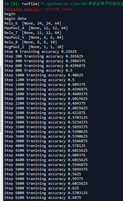
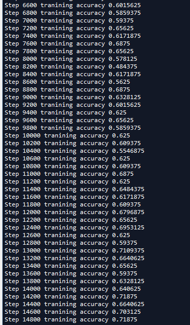
我们可以看到这个模型准确率接近70%，这主要是因为我们在图像预处理是进行了输入归一化处理，导致比我们在第十六节，卷积神经网络之AlexNet网络实现(六)文章中使用传统神经网络训练准确度52%要提高了不少，并且比AlexNet的60%高了一些(AlexNet我迭代的轮数比较少，因为太耗时)。 

完整代码：

# -*- coding: utf-8 -*-
"""
Created on Thu May  3 12:29:16 2018

@author: zy
"""

'''
建立一个带有全局平均池化层的卷积神经网络  并对CIFAR-10数据集进行分类
1.使用3个卷积层的同卷积操作，滤波器大小为5x5，每个卷积层后面都会跟一个步长为2x2的池化层，滤波器大小为2x2
2.对输出的10个feature map进行全局平均池化，得到10个特征
3.对得到的10个特征进行softmax计算，得到分类
'''

import cifar10_input
import tensorflow as tf
import numpy as np


'''
一 引入数据集
'''
batch_size = 128
learning_rate = 1e-4
training_step = 15000
display_step = 200
#数据集目录
data_dir = './cifar10_data/cifar-10-batches-bin'
print('begin')
#获取训练集数据
images_train,labels_train = cifar10_input.inputs(eval_data=False,data_dir = data_dir,batch_size=batch_size)
print('begin data')


'''
二 定义网络结构
'''
def weight_variable(shape):
    '''
    初始化权重
    
    args:
        shape：权重shape
    '''
    initial = tf.truncated_normal(shape=shape,mean=0.0,stddev=0.1)
    return tf.Variable(initial)

def bias_variable(shape):
    '''
    初始化偏置
    
    args:
        shape:偏置shape
    '''
    initial =tf.constant(0.1,shape=shape)
    return tf.Variable(initial)


def conv2d(x,W):
    '''
    卷积运算 ，使用SAME填充方式   池化层后
         out_height = in_hight / strides_height（向上取整）
         out_width = in_width / strides_width（向上取整）
    
    args:
        x:输入图像 形状为[batch,in_height,in_width,in_channels] 
        W:权重 形状为[filter_height,filter_width,in_channels,out_channels]        
    '''
    return tf.nn.conv2d(x,W,strides=[1,1,1,1],padding='SAME')


def max_pool_2x2(x):
    '''
    最大池化层,滤波器大小为2x2,'SAME'填充方式  池化层后
         out_height = in_hight / strides_height（向上取整）
         out_width = in_width / strides_width（向上取整）
    
    args:
        x:输入图像 形状为[batch,in_height,in_width,in_channels] 
    '''
    return tf.nn.max_pool(x,ksize=[1,2,2,1],strides=[1,2,2,1],padding='SAME')
    

def avg_pool_6x6(x):
    '''
    全局平均池化层，使用一个与原有输入同样尺寸的filter进行池化，'SAME'填充方式  池化层后
         out_height = in_hight / strides_height（向上取整）
         out_width = in_width / strides_width（向上取整）
    
    args；
        x:输入图像 形状为[batch,in_height,in_width,in_channels] 
    '''
    return tf.nn.avg_pool(x,ksize=[1,6,6,1],strides=[1,6,6,1],padding='SAME')

def print_op_shape(t):
    '''
    输出一个操作op节点的形状
    '''
    print(t.op.name,'',t.get_shape().as_list())


#定义占位符
input_x = tf.placeholder(dtype=tf.float32,shape=[None,24,24,3])   #图像大小24x24x
input_y = tf.placeholder(dtype=tf.float32,shape=[None,10])        #0-9类别 

x_image = tf.reshape(input_x,[-1,24,24,3])

#1.卷积层 ->池化层
W_conv1 = weight_variable([5,5,3,64])
b_conv1 = bias_variable([64])


h_conv1 = tf.nn.relu(conv2d(x_image,W_conv1) + b_conv1)    #输出为[-1,24,24,64]
print_op_shape(h_conv1)
h_pool1 = max_pool_2x2(h_conv1)                            #输出为[-1,12,12,64]
print_op_shape(h_pool1)


#2.卷积层 ->池化层
W_conv2 = weight_variable([5,5,64,64])
b_conv2 = bias_variable([64])


h_conv2 = tf.nn.relu(conv2d(h_pool1,W_conv2) + b_conv2)    #输出为[-1,12,12,64]
print_op_shape(h_conv2)
h_pool2 = max_pool_2x2(h_conv2)                            #输出为[-1,6,6,64]
print_op_shape(h_pool2)



#3.卷积层 ->全局平均池化层
W_conv3 = weight_variable([5,5,64,10])
b_conv3 = bias_variable([10])

h_conv3 = tf.nn.relu(conv2d(h_pool2,W_conv3) + b_conv3)   #输出为[-1,6,6,10]
print_op_shape(h_conv3)

nt_hpool3 = avg_pool_6x6(h_conv3)                         #输出为[-1,1,1,10]
print_op_shape(nt_hpool3)
nt_hpool3_flat = tf.reshape(nt_hpool3,[-1,10])            

y_conv = tf.nn.softmax(nt_hpool3_flat)

'''
三 定义求解器
'''

#softmax交叉熵代价函数
cost = tf.reduce_mean(-tf.reduce_sum(input_y * tf.log(y_conv),axis=1))

#求解器
train = tf.train.AdamOptimizer(learning_rate).minimize(cost)

#返回一个准确度的数据
correct_prediction = tf.equal(tf.arg_max(y_conv,1),tf.arg_max(input_y,1))
#准确率
accuracy = tf.reduce_mean(tf.cast(correct_prediction,dtype=tf.float32))


'''
四 开始训练
'''
sess = tf.Session();
sess.run(tf.global_variables_initializer())
tf.train.start_queue_runners(sess=sess)

for step in range(training_step):
    image_batch,label_batch = sess.run([images_train,labels_train])
    label_b = np.eye(10,dtype=np.float32)[label_batch]
    
    train.run(feed_dict={input_x:image_batch,input_y:label_b},session=sess)
    
    if step % display_step == 0:
        train_accuracy = accuracy.eval(feed_dict={input_x:image_batch,input_y:label_b},session=sess)
        print('Step {0} tranining accuracy {1}'.format(step,train_accuracy))